Abstract

Chains of amino-acids, i.e. proteins, are an essential building block of life that can carry out many useful functions for medical and industrial applications. The ability to extract information from protein sequences and to predict the effects of mutations is extremely valuable in many domains of biology and medicine. Designing proteins that are able to catalyze specific biochemical reactions is a major challenge tackled through computational methods as well as directed evolution, strategies that made huge improvements since the 1970 but are still faced with the intractability of exploring the gigantic space of all possible proteins.
Recently, Generative Models such as GANs (Generative Adversarial Networks) and VAEs (Variational Auto Encoders) have been used successfully to model the distribution of images and to generate novel, realistic samples. Conditional Models have been used to generate samples with desired high-level features when annotated data is available, for instance here.
Here, we demonstrate the ability of such networks to generate novel proteins that have expected biochemical properties. In a first part, we use a computational model associated to a folding-related fitness metric to assess the quality of novel proteins generated by different models. We then build a Conditional VAE with an autoregressive decoder, inspired by the WaveNet architecture, that we call the ProtCNN. After training on a dataset of 70000 luciferase-like oxidoreductases, a set of proteins sharing a common biochemical activity, we show that the model is able to learn meaningful information such as amino-acid relatedness and can generate novel proteins when conditioning upon high level properties such as charge, molecular weight or solubility. We also introduce a fitness metric for the structure of the protein and show that our model is able to generate variants of a protein that have a consistent secondary structure. We believe that this type of model provides an intelligent way to explore the space of possible proteins and hope that the methods presented here will pave the way for new powerful tools to generate protein variants.

Acknowledgements

I want to thank David Bikard, my internship supervisor and head of the synthetic biology lab at Institut Pasteur, for his valuable support. Many thanks to Sebastien Baur for starting this project, and to Jerome Wong Ng and Alexander Hawkins Hooker for fruitful discussions.

The work presented here used the computational and storage services (TARS cluster) provided by the IT department at Institut Pasteur, Paris.

Code available here.

Introduction

Protein Design

Proteins are large biomolecules, organized in long chains of amino acid residues, that perform many biological functions within organisms, among which DNA replication, metabolic reactions catalysis, converting various sources of energy (light, chemical gradients...), and transporting molecules from one place in the cell to another. Proteins also have a wide range of therapeutic, medical and industrial applications: industrial enzymes are used to produce food, biofuels, chemical and pharmaceutical products; recombinant proteins have medical applications involving vaccines and antibodies. In many of these applications, it is often desirable to modify properties of natural proteins to remove some disturbing side reaction or increase catalytic activity.

Protein design is the art of designing new molecules that have expected behaviors and biological functions, for instance ability to fold into specific structures and catalyze biochemical reactions. Directed evolution is a straightforward method to increase the fitness of a protein, that mimics the process of random mutation and natural selection ^[1]. However this process is quite slow and only explores a fraction of all possible proteins, so rational protein design began in the 1970's. Since then, it has made tremendous progress thanks to advances in molecular forcefields and bioinformatics, which paved the way for advanced computational protein design tools. In 2017, the global protein engineering market size was valued at about 1,000,000,000$, with an annual growth rate of about 16%.

Rational protein design can be performed from scratch (de novo protein design), a field that made some progress recently^[2]. Most of the time however, protein design starts from existing proteins whose structure is already known ^[3], and aims at identifying interesting mutations.

The properties of a protein highly depend on the spatial organization of its amino-acid chain. The amino acid residues of a protein interact with one another and with the external environment, causing the protein to fold into particular 3D structures in which it can fulfill its biological function. This process is called Protein Folding. Misfolded proteins are generally inactive, but might sometimes have modified or toxic functionality. For instance, many allergies are caused by proteins that acquire a non-native folding, because our immune system can produce antibodies for only certain protein structures.

Left: Amino-Acid Sequence, Right: Representation of folded protein

Many chemical interactions are involved in the process of protein folding, including hydrophobicity, acidity, and hydrogen bonding effects. The relationship between the primary structure of a protein (its amino-acid sequence) and its native folding is only partly understood because of the complexity and the scale of atom-to-atom interactions. The problem of finding the 3D folding of a protein is extremely challenging due to severe computational limits on all-atoms simulations. Protein folding softwares, like RaptorX, exploit amino acid interactions as well as homologies with proteins for which the 3D structure has been determined through physical methods (NMR Spectroscopy and X-ray crystallography). Computer-aided protein design can help identify interesting mutations, but the difficulty to predict protein fold and function make it hard to create functional variants of a protein.

This limitation associated with the gigantic space of the protein sequence space makes a systematic exploration of protein variants intractable: Indeed, the human DNA directly encodes 20 different amino-acids, resulting in a protein space size of 20³⁰⁰ for a fixed amino-acid chain length of 300, which is an average size for a protein.

A smart way to explore the protein space is therefore needed to generate functional variants that have interesting properties. Machine Learning methods are being reviewed for that purpose. A few recent studies have explored deep neural networks to model chemicals represented as SMILES strings in order to propose novel interesting molecules likely to have desired activities ^{[4] [5] [6]}. In a recent paper ^[7], variants of the green fluorescent protein (GFP) are made using supervised learning : The fitness function (light emission property) is being learned by a neural network, and new variants are being generated by Monte Carlo Sampling, interpreting the output of the model as energies.

Here, we make use of deep generative models, which offer extremely promising tools for the exploration of low-dimensional manifolds in high-dimensional spaces.

Variational Auto Encoders

In Machine Learning, Generative Models are statistical models that given on observable variable $X$, are able to sample data from the distribution of $X$.
Auto Encoders are neural networks, composed of an encoder network, that encodes the protein into a low dimensional vector space called the latent space, and a decoder that reconstructs the protein from its latent space representation. The network is then trained end-to-end using backpropagation. This principle is called an information bottleneck, and it forces the network to encode only the most important features of a protein into the latent space, that will allow for a faithful reconstruction of the protein. The identity function is learned in a non-trivial way, forcing the latent space to represent high-level features about the data.

To help the network learn meaningful information in the latent space and reduce overfitting, Variational Auto Encoders ^{[8] [9]} are used. In a VAE, the distribution of the encoded data in latent space is forced to follow a normal distribution via a KL-divergence loss term. As a result, most areas of the latent space can be decoded into valid samples, and it is possible to adjust the level of each feature independently by sampling the latent space.
For instance, when trained on faces, the VAE learns features such as hair color, presence of glasses, shape of the head, that can be changed manually by modifying the encoded representation of an image ^{[10] [11] [12]}. Moreover, it is possible to perform arithmetic operations and interpolation on the encoded vectors, which produces vectors that can be decoded to novel samples.

Metrics for Proteins

Since the distribution of the input dataset is generally unknown, it is difficult to assess the quality of samples coming out of generative models. Two natural techniques for this purpose are whether humans, or adversarial networks, can tell the difference between the real data and the generated data ^[13].

When generating new molecules, specific metrics exist, such as the Fréchet ChemblNet Distance ^[14]. The authors claim that the FCD can detect if generated molecules have similar chemical and biological properties as real molecules, and are distant enough from one another.

In this work we are going to focus in particular on to what extent a protein sequence can be mutated without removing its biological function. We will therefore discuss fitness functions related to biological activity to assess functionality, along with distance functions between proteins to assess how different a variant is from the original protein.
The former is much more complicated than the latter as physical measurements, or at least simulations are involved in the calculation of functionality, and such fitness metrics will be defined throughout this work. For the distance between proteins, it is often sufficient to use the alignment metric, which is the edit distance between the sequences of theses proteins (number of insertions, deletions, and mismatches needed to go from a sequence to the other). This metric is fairly satisfying as it reflects quite well the process of natural evolution. In this metric however, properties of amino-acids are not taken into account, and swapping amino-acids with similar properties is much more likely to have no impact on the protein's activity than swapping dissimilar amino-acids (positively charged and negatively charged for instance). This phenomenon is captured in the Blosum 62 Matrix $B_{62}$ ^[15], which for two amino-acids $a$ and $b$ indicates the level of interchangeability of those two amino-acids $B_{62}[a, b]$. This matrix is computed from alignments of sequences in families of proteins, and the '62' is a filter parameter in this computation.
The higher the Blosum score of two amino-acids, the more easily one can be replaced by the other in a protein sequence without disturbing its structure. A high score for $B_{62}[a, a]$ indicates that amino-acid $a$ has specific properties and therefore is not easily swappable.

We define the B62 distance, which is the edit distance where the cost of a mismatch $a \leftrightarrow b$ is $B_{62}[a, a] - B_{62}[a, b]$. This correction makes sense from a chemical point of view compared to the original edit distance; we will often use the two metrics for comparison.

Benchmarking Generative Models with Lattice Proteins

Here, we present an evaluation method for generative models, based on Lattice Proteins ^[16], which has been used to evaluate Restricted Boltzmann Machines ^[17]. We demonstrate the relevance of this metric and show that Variational Auto Encoders can be tuned to generate relevant and diverse proteins, outperforming statistical and blosum-inspired models.

Lattice proteins are highly simplified models of proteins, for which the computational effort in handling the model is significantly reduced, although still NP-complete. In the Lattice Protein model, foldings are regarded as paths into multi-dimensionnal grids, called structures:

A path into a 3 x 3 x 3 cubic lattice

From now on we will only consider paths of size 27 on this 3 x 3 x 3 cubic lattice. There are 103,406 possible structures on this lattice, excluding symmetries, on which a protein composed of 27 amino acids can be folded. Physical interactions between amino acid residues are calculated for residues occupying neighbouring sites on the lattice. Interaction energies for neighbouring amino acids are given by the Miyazawa-Jernigan Energy Matrix ^[18] $E$: The energy of a sequence $A = (a_1, a_2, ... a_{27})$ folded into a structure $S$ is
$\mathscr{E}(A\vert S) = \sum_{i<j} c_{i, j}^{(S)} E_{i, j}$
where $c_{i, j}^{(S)}$ is the contact map associated to the structure $S$: $c_{i, j}^{(S)} = 1$ if the amino acids at positions $i$ and $j$ in the protein sequence are on neighbouring sites in the lattice.

Fitness score for lattice proteins

A Sequence $A$ will natively fold into a structure $S$ with a Boltzmann probability that depends on the folding energies on all lattice structures: for unit temperature,
$P_{nat}(S\vert A) = \frac{e^{-\mathscr{E}(A, S)}}{\sum_{S'} e^{-\mathscr{E}(A, S')}}$

The sequences $A$ that have a high probability of folding into structure $S$ are sequences such that they present large gaps between their folding energy in $S$ and their folding energies in all other structures $S'$.

Through Monte Carlo Simulations^[16:1],[19], it is possible to create a list of sequences $A_1, .. A_n$ that have a very high probability (e.g. 0.995) of folding into one specific structure $S$. Starting from a arbitrary sequence $a_1, .., a_{27}$, the simulation attempts to make mutations $a_i \rightarrow a_i'$, which are accepted if the new folding probability $P_{nat}(S\vert A')$ is higher, and accepted with probability $(P_{nat}(S\vert A')/P_{nat}(S\vert A))^{\beta}$ otherwise, where $\beta$ plays the role of an inverse temperature, which helps the simulation escape local minimas in the energy function.

It is also possible to add a bias term in the corresponding Hamiltonian to account for phylogenetic effects in sequence mutation^[16:2].

The resulting sequences share a non-trivial high-order folding property while being very different from one another. The folding score into the structure $S$ can therefore be seen as an evaluation metric for generative models.

Methods

H. Jacquin, A. Gilson, E. Shakhnovich, S. Cocco, & R. Monasson made available four lists of proteins that fold natively into four lattice structures, that is available for download here.

Hereafter, we consider the lattice structure $S_0$ with its list of ~ 50,000 proteins of size 27 that fold into $S_0$ with probability $p$ > 0.99.

We implement a variational auto-encoder (VAE) that learns a compressed representation of this dataset of proteins, and then generate new proteins by sampling the latent space distribution. We then score the generative model based on three metrics:

• The folding score of the generated sequences. For convenience, we use for each sequence $A$ the scoring function $f(A) = - ln(1-P_{nat}(S_0\vert A))$
• The smallest edit distance between a generated sequence and the train dataset.
• The histogram of pairwise distances in the generated sequences.

Indeed, a good generative model should be able to generate sequences that fold into structure $S_0$, while being significantly different from the dataset. Moreover, the pairwise distances distribution of the generated sequences should correspond to the one of the original dataset.

We use the following baseline models to assess the relevance of Variational Auto Encoders:

• Blosum Model: The Blosum 62 Matrix indicates which amino-acids can easily be replaced by one another in the sequence of a protein. Therefore, we can use this matrix to generate variants of a protein, by choosing some positions and changing the amino-acids at those positions to closely related amino-acids.
• MSA Model: In a multiple sequence alignment, it is critical that some positions are occupied by a particular amino-acid. We can use this property to generate variants: For each position $i$, we can decide to change the amino-acid at this position to another one by sampling the distribution of amino-acids at this very position.

We study a Variational Auto-Encoder with 5 layers (including input and output layers), that we call VAE$_{10}$. Below is the graph of this VAE: In each cell are indicated the size of the layer (number of artificial neurons).

where z_sample is sampled from a gaussian distribution with mean $z_{meam}$ and variance $e^{z_{log\_sigma}}$:
$z_{sample} \sim \mathscr{N}(z_{mean}, e^{z_{log\_sigma}})$

We will also review a VAE with the same structure and more parameters, the VAE$_{30}$:

These networks are trained with a loss $L = L_{cross\_entropy} + L_{KL\_div}$^[8:1], with
$L_{cross\_entropy}(x, x') = x log(x')$ $L_{KL\_div} = \frac{1}{2}(z_{mean}^2 + e^{z_{log\_sigma}} - z_{log\_sigma} - 1)$

Roughly speaking, the first term is the reconstruction accuracy between a protein $x$ and its reconstructed sequence $x'$: The lower the loss, the closer $x$ and $x'$ are.
The KL Divergence loss measures how far the distribution of the latent variable $z_{mean}$ is from a gaussian distribution $\mathscr{N}(0, 1)$.

By minimizing the loss $L$, the model both learns to reconstruct the proteins of the training set and to model these proteins with a latent distribution that is close to a gaussian distribution $\mathscr{N}(0, 1)$.

A new variant of a protein $x$ is then calculated with the following algorithm

• compute $z_{mean}$ and $z_{var}$ with the encoder network
• sample $z = z_{mean} + r * z_{var}$ where $r \sim \mathscr{N}(0, s)$
• Decode $z$ into a new protein $x'$ with the decoder network.

The parameter $s$ is the sampling factor. During training, $s = 1$, but during test time, we can take larger values of $s$ to generate more distant variants.

Results

Here, we show a scatter plot of the data generated with the Msa Model, the blosum Model, the VAEs with a latent space of size 10 and 30, and some data from the original protein dataset kept as test dataset. The parameter stddev corresponds to the sampling factor $s$ during generation of variants for the VAEs. Each point (x, y) in the graph is a variant $A$ of a protein in the training set, where x is the smallest edit distance to the proteins of the training set and y is the folding score $f(A)$ relative to the structure $S_0$. Across different generative models, points are slightly shifted on the x axis to improve visibility.

• The baseline models gives very poor results: The generated sequences fail to fold natively into the structure $S_0$. Only 6% of the sequences generated with the blosum model fold into $S_0$ with probability higher than 85%. The MSA Model is slightly better with 25% generated sequences folding with a probability higher than 85%. These models are very far from the sequences scores of the test dataset, as expected, due to the complexity of the metric.
• The Two Variational AutoEncoders, tested with a sampling factor of 3, give different results: They are both able to generate high-quality sequences that fold into $S_0$ with probability >98% for 98% of them. However, the more complex VAE with a latent space of size 30 generates samples that are closer to the training set: Indeed, this network is able to better reconstruct the input sequences, with a reconstruction accuracy of 85%. The VAE$_{10}$ has a reconstruction accuracy of only 53%, but this does not impact the folding score of its generated sequences. As a result, these sequences are quite distant from the training set, with a minimum Hamming Distance of 11 on average, which corresponds to a maximum sequence homology of 60% between a protein and its closest sequence in the training set.
• It is possible to obtain more distant variants with the VAE$_{30}$ by increasing the sampling factor up to 25. The generated sequences are then more distant from the training set, but this has a drastic impact on the folding score: Only 35% of the proteins are able to fold correctly with a probability of 98%, and 13% have a folding probability below 85%.

From the above remarks, we understand that:

• Statistical Methods and bio-inspired methods fail to generated sequences that have the same folding property as the training sequences.
• The quality of reconstruction is not a good metric regarding the goal of generating sequences that are both distant from the training set and have a good folding score.
• A smaller latent space size for a VAE can help to capture a simpler representation of the training sequences without affecting the folding score.

Variants Diversity

The VAE$_{10}$ models the data distribution correctly with respect to the folding metric and is able to generate new proteins distant from the training set. But are the generated samples distant from one another ? Here, we compute the pairwise distance between the generated samples, and compare it with the "true" pairwise distance distribution of the test dataset. Distances are evaluated using the B62 distance, as discussed in the introduction.
Here is the histogram of pairwise distances between proteins, for the test dataset and for the Auto Encoder variants.

We can see that the VAE$_{10}$ model generates samples that are as diverse as the original set of proteins, which is what we desired.

Generating variants of Luciferase Enzymes

We have seen that Variational Auto Encoders with a simple architecture are able to model complex distributions and preserve the structure of a protein in the Lattice Proteins Model, as measured by the folding accuracy metric. However, in this model, all the proteins have a fixed size of 27 amino-acids, which is not biologically relevant: In reality, most proteins have a length of hundreds, sometimes thousands of amino-acids. We will now study a much more complex family of real-life proteins: the Luciferase domain, a group of enzymes that all catalyze the same bio-chemical reaction, which can in some cases produce light. We will model the distribution of these proteins with a more complex VAE, and will try to assess whether this model generates interesting proteins by investigating its ability to understand basic properties about amino-acids and extrapolate the general folding structure of the Luciferase domain.

Background

The Bac Luciferase Family

Luciferase is a generic term for the class of oxidative enzymes that produce bioluminescence. They are found in a variety of organisms, including fireflies, jellyfish and bacteria. Luciferases catalyze a chemical reaction which consumes a substrate called luciferin and produces a blue-green light. Luciferases can be produced in the lab through genetic engineering for a number of purposes. Photo emission can be detected by appropriate light detector, which allows for observation of biological processes, among other things.

Luciferase are organized, as all other proteins, in a hierarchy representative of the natural evolution. A protein family is a set of proteins that share a common ancestor, reflected by their related functions and similarities in sequences and structure. Families of proteins that display a common evolutionary origin are called superfamilies. Databases of the Luciferase superfamily can be found online on PFAM (PF00296) and INTERPRO (IPR011251). These databases are build based on sequence identity, and gather proteins responsible for a unique oxidative process that does not always result in light emission. It means that most proteins in the dataset do not effectively produce light and it might also be that they catalyze side-reactions.

Moreover, there is a high sampling bias in this dataset: some proteins have a high sequence homology, which is defined as the percentage of amino-acids that two proteins have in common (after alignment). We call a cluster50 a set of proteins that have a pairwise sequence homology of more than 50% and a cluster90 a set of proteins that have a pairwise sequence homology of more than 90%. When not specified, a "cluster" will refer to a cluster50.

Modern Auto-Encoders

We already presented Variational Auto Encoders, that learn a compressed and meaningful representation of a dataset through an information bottleneck. When generating images, VAEs capture the global structure of the data, but the images they generate by sampling the latent space tend to be blurry as high-frequency details in the input images (edges, textures...) tend to disappear because they do not carry enough information. To solve this issue, it has been proposed to use an autoregressive decoder in a VAE ^[20]. In an autoregressive model, each pixel is generated as the next element in a sequence, given both the latent vector of the image and the previously generated pixels: the joint data distribution is modeled as $\mathbb{P}(X\vert z) = \prod_{i=1}^N \mathbb{P}(x_{i+1} \vert z, x_1, ..., x_i)$
Autoregressive models, such as Recurrent Neural Networks (especially LSTM and GRU architectures ^{[21] [22]}) have been used to model long range dependencies in time series but they are quite long to train, Alternatively, causal (or masked) convolutions offer a convenient framework to model sequences with long-range dependencies, with a comparable performance while being trainable much faster in parallel ^[23]. Causal convolutions ensure that prediction of a point only depends on the previous point ^{[24] [25] [26]}.

Another major improvement to classical VAE is the possibility to remove some high level features from the latent space and pass them as extra-parameters, when the dataset is annotated with these high-level features. After training, one can then manually change these high-level features to produce samples with desired properties. This is called conditioning.

Finally, it has been shown that the use of gated activation functions ^{[24:1] [27]} can substantially increase performance.

We present here a conditional VAE, whose decoder is an autoregressive model strongly inspired by the Wavenet architecture ^{[20:1] [28]}. We will condition the generated sequences upon some physical properties of the proteins that are not directly encoded in the amino-acid sequence but calculated via an external software.

Model Details

Architecture

The architecture of our model is the following:

The vector x is a one-hot encoding of the protein: With 21 amino-acids (including a padding character) and a length of 300, the one-hot encoding have a shape of (300, 21).
The vector c contains the physical quantities of the protein we condition upon: the length of the protein, its charge, its isoelectric point, its molar extinction coefficient, its solubility, and its molecular weight. These quantities are estimated using the pepstats tool from the EMBOSS software suite ^[29], and then normalized to have null mean and unit variance.
During training, the vectors x and c are encoded into a latent space variable z. z is then upsampled conditioning on c, generating z' which is then passed to the autoregressive model that reconstructs x'.

The encoder network has the following architecture:

All convolutions have a stride of 2, and the number of filters is doubled each time. The Sample Layer computes $z = z_{mean} + r * z_{std}$ where $r \sim \mathscr{N}(0, s)$.

The UpSampling Network is

The fully connected part contains information about the protein features while the deconvolutional part adds information about the location these features. Doing both rather than just one improves test reconstruction accuracy by 1%.

The Decoder Architecture has the following architecture:

where each WaveNet block is

All the residual connections are added together at the + Node. These residual connections reduce the vanishing gradient problem , making the training easier ^[30]. Here, only three WaveNet blocks are represented, but there could be a chain of $k$ WaveNet blocks. Causal convolutions are convolutions that map an input sequence $s$ to an output sequence $s'$ of same size. Each element in the output sequence only depends upon the corresponding previous elements in the input sequence. Each causal convolution is dilated with a dilation factor doubled each time, so that the receptive field of the autoregressive model grows exponentially with the number of WaveNet blocks. After 3 blocks, the receptive field is 32 amino-acids.

Hyperparameters and Reconstruction procedure

All convolutional layers have a kernel size of 2 and are followed by batch normalization, a very effective technique to improve reconstruction accuracy while dramatically increasing training speed ^[31]. When not specified, the layers are followed by a PReLU Activation Layer (Parametric Rectified Linear Unit), which yielded the best reconstruction performance (tested against ELU, ReLU, tanh) ^[32].

We train the ProtCNN network as a typical VAE network, with a loss composed of a KL-divergence term and a cross-entropy term. The loss is minimized using the Adam optimizer^[30:1] with default parameters for 50 epochs.

The generation of a one-hot encoded protein from a latent vector z and a conditions vector c is done with the following algorithm:

x = array of zeros with shape (prot_size, 21)
for i=1..prot_size do
p <- Decoder([x, z, c])[i, :]  # Amino-acid probabilities for position i
x[i, argmax(p)] <- 1  # The most probable amino-acid is set at position i

Model Analysis

Accuracy Results

When trained of the Luciferase-like (LL) protein dataset with a random train/test split, the model predicts the next amino-acid in a sequence with a 77% test accuracy. However, since some sequences in the dataset are very close from one another, we can build a test set where the maximum homology between a protein from the train set and a protein from the test set is 50%. In that case, the model predicts the next amino-acid in a sequence with a 62% accuracy. Trying to reconstruct proteins that are not in the LL domain led to accuracies close to 12%, which means that the model learns features that are specific to the LL domain.

Distribution of Amino-Acids and n-grams

In proteins, amino-acids are not equally distributed and some appear more often than others. We expect the neural network to generate sequences with the same amino-acid frequencies that in the training dataset. Moreover, groups of three amino-acids (called 3-grams or 3-mers) also do not occur with uniform probability in the dataset. We can therefore compare the frequencies of occurrence of the 8397 unique 3-mers in the training set and in the sequences generated by sampling the latent space.

Here are the results:

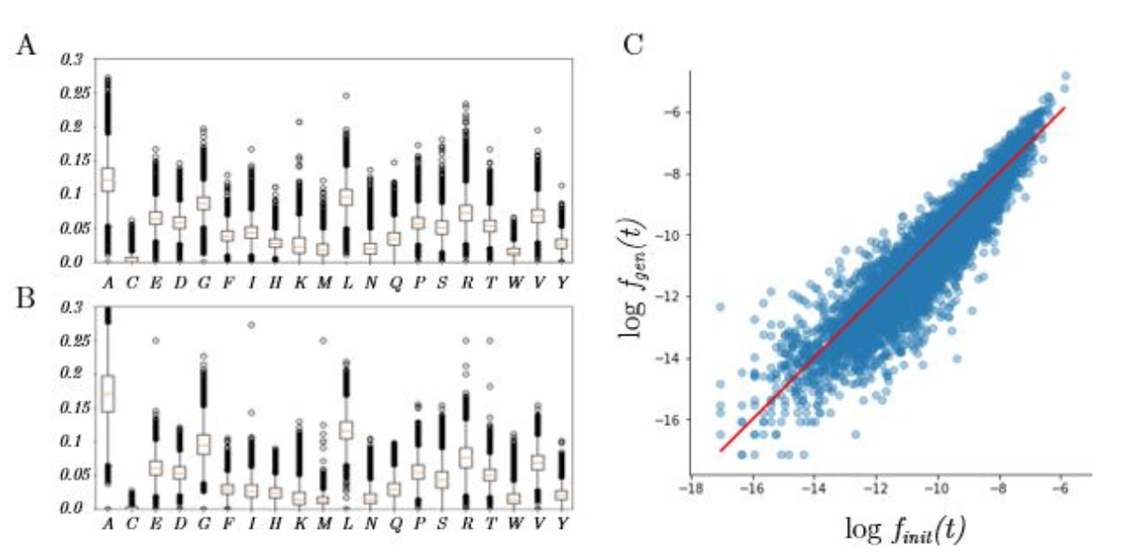
Left: Distribution of amino-acid frequencies, for the training dataset (A) and the generated sequences (B).
Right: Scatterplot of the probabilities of occurence of the 3-mers (x-axis: training set, y-axis: generated sequences)

As we can see, the generative network can indeed roughly reproduce the distribution of amino-acids, but it tends to predict abundant amino-acids such as Alanine (A) too frequently and rare amino-acids such as Cysteine $C$ too rarely. This problem of imbalanced classes is standard in classification problems ^[33] and can be solved by a weighted loss associated to each amino-acid, which might be considered for future work.
While the 3-gram frequencies of the generated sequences correlate nicely with the training set, we can observe the same tendency to produce abundant 3-grams more often than expected.

Latent Space Organization

During training, the KL divergence term encourages the encoded data in the latent space to follow a normal distribution $\mathscr{N}(0,1)$. The true distribution is however not normal and some regions of the latent space are left "empty", far from the reconstructed proteins. As a result, when sampling the latent space randomly, only 30% of the generated sequences are identified as part of the bacterial Luciferase like PFAM family, where the identification is made with a Hidden Markov Model with a E-value score filter of 0.1.

When training the latent space without conditioning, the latent space encoded physical properties of the protein, the principal component being strongly correlated with the protein size for instance. With conditioning, the correlation between the latent space variables and the properties passed as a conditioning vector is strongly reduced.

The latent space tends to group together proteins than belong to the same family. Indeed, we identified 24 relatively balanced non-overlapping Interpro families containing more than 100 samples, for a total of 50 000 proteins, inside the Luciferase domain. A simple multi-class logistic regression model trained on top of the latent representation of these 50 000 proteins allows to classify proteins with a 92.7% accuracy. This shows that the different families tend to be well separated in the latent space.

Amino Acid Relatedness

Along with the preservation of the statistical distribution of the dataset, a natural question is whether the network is able to learn sensible biological information about proteins. One way to assess this is to check whether the network captures the notion of amino-acid interchangeability: amino acids having similar properties (charge, polarity, hydrophobicity, weight...) are more likely to preserve the activity and folding of a protein when swapped in its sequence, as quantified by the Blosum 62 matrix.
When the ProtCNN network reconstructs a protein, it outputs for each protein and each sequence position a set of 21 probabilities, one for each amino-acid. Close amino-acids are likely to have similar probabilities in these sets of probabilities. That is why we can compute for two amino acids $a$ and $b$, the correlation coefficient of the probabilities associated to $a$ and $b$ across all positions and all proteins.

This correlation coefficient is high if $a$ and $b$ are highly swappable and low otherwise. The values of these coefficient seem to be have a non-linear (second-order polynomial) relation with the Blosum Matrix. Correcting this non-linear effect give us a new Blosum 62 matrix whose values are comparable to the original Blosum 62 Matrix.

We visualize these generated values with a scatterplot, to check the relationship between the new blosum values and the original Blosum 62 values, and a heatmap, where hot colors indicate high interchangeability and cold colors low interchangeability.

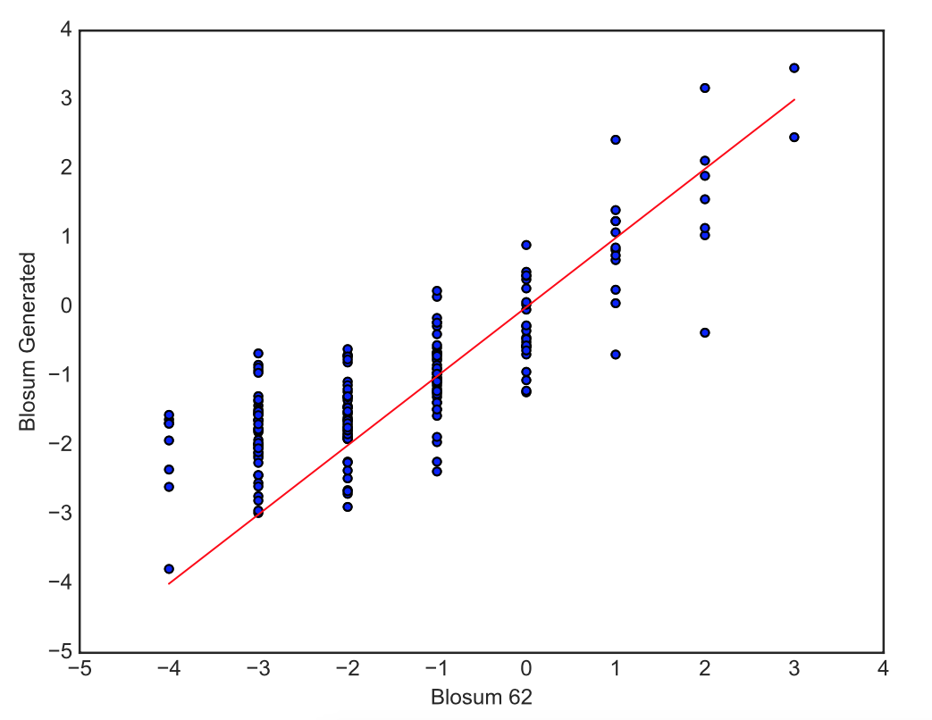> Right: Scatterplot of the generated blosum values versus the original Blosum 62 values for all pairs of amino-acids. > Left: HeatMap of Blosum Values. Lower Diagonal: Original Blosum 62 Matrix, Upper Diagonal: Blosum Matrix generated with the correlation coefficients. The amino-acids in the x and y axis are represented by their letter and are ordered so that amino-acids with similar properties are close to each other.

We can see a strong correlation between the original values and the generated values. The upper diagonal (Generated Blosum) of the heatmap has the same general structure as the lower diagonal (Original Blosum).

Our model therefore understands very well the similarities and dissimilarities of amino-acids, with the notable exception of W and Y that are not predicted as easily swappable by our model although identified as such by the Blosum 62 Matrix.

Conditioning

Conditioning consists in providing additional information to the encoder and the decoder, which allows to control the high-level features of the generated samples. In our case, the high-level features are physical properties of the proteins: the length, charge, iso-electric point, molar extinction coefficient and probability of expression in inclusion bodies, which is a measure of solubility. Interestingly, providing these information enabled a 2% gain in reconstruction accuracy.

To test the ability of our model to generate samples with desired properties, we consider a set of fixed properties and let one condition vary linearly from -2 to +2 (quantities are standard scaled). We then sample 32 points from the latent space with these conditions and generate the corresponding proteins, for which we then re-calculate the physical properties to check if the conditioning worked. It is worth noting than we cannot condition on very correlated variables (such as length and molecular weight) independently.
Here, we show an example of a conditioning graph where we condition upon solubility. The green lines represent the value provided in the conditioning vector:

We can see that the physical properties of the reconstructed proteins are well conserved on average, but there is a lot of variance in the results.

Next, we chose a specific protein (a F420-dependent glucose-6-phosphate dehydrogenase) and generated variants of this proteins by conditioning upon increasing values of solubility (decreasing values of insolubility). Although conditioning did not work perfectly, it produced significant results on the solubility parameter without affecting the other physical properties.

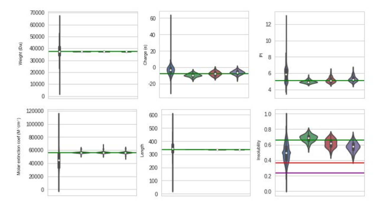> Blue violins: Distribution over the whole dataset. The following violins are obtained by generating 100 variants of the input protein, with no conditioning (Green), conditioning with insolubility of 0.39 (Red), and conditioning with solubility of 0.22 (Purple). The corresponding green, red and purple lines show the theoretical values on expectation.

Secondary Structure Conservation

The protein secondary structure is the 3D organization of local segments of amino-acids in the protein sequence. The two most common secondary structural elements are the alpha helix, and the beta sheet (formed of beta strands).
Below is a simplified representation of those two elements.

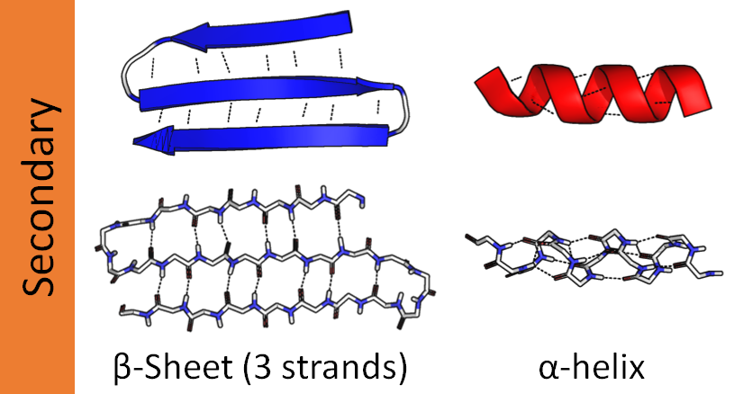
Secondary structure elements typically spontaneously form as an intermediate before the protein folds into its native 3D structure (tertiary structure).

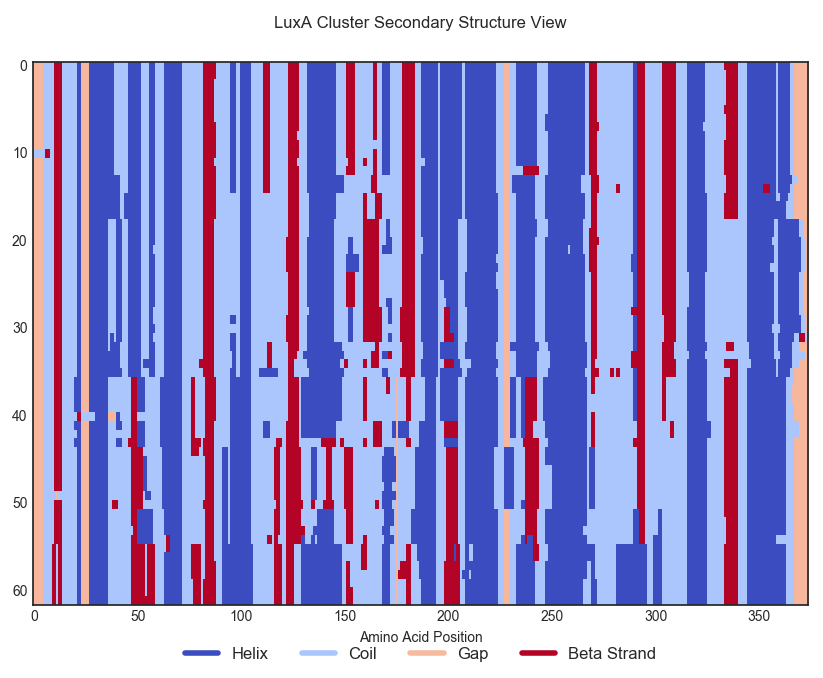
In this section, we want to check whether our generative model can make functional variants of a protein, for which it is needed that the variants have the same structure as the original protein and in particular the secondary structure. We will especially focus on a protein called LuxA and its cluster of closely related proteins.

Computing the secondary structure of a protein is a simpler problem than computing the whole 3D structure but is still very challenging. Most softwares need a multiple sequence alignment from a protein family to compute the secondary structure of all the proteins in the alignment, assuming that they all have the same spatial organization. However we cannot use this technique to compute the secondary structure of our variants because the software will see our mutations as noise and will output an averaged secondary structure close to our original protein in any case. That is why we use the PSIPRED software ^[34] for computing secondary structures for single proteins, which has the unavoidable drawback of having a lot of noise in its output. PSIPRED gives, for each amino-acid in a sequence, the probability that this amino-acid is part of an helix ($p_H$), a beta strand ($p_E$) or a coil ($p_C$), with $p_C + p_H + p_E = 1$, along with the most probable secondary structure element for this amino-acid. From now on, we say that a sequence S= 'CCCCHHHHEECCC...' is the secondary structure of a protein $p$ if each character in S represents the structure of the corresponding amino-acid in the protein sequence, as computed by PSIPRED.

Here is a colored view of the secondary structure of the proteins in LuxA's cluster. Each row corresponds to a protein in this cluster, and each column to a position in the sequence alignment. Proteins have been aligned and re-ordered to improve legibility.

Changing random amino-acids at random places often spoils the secondary structure of a protein as it can remove essential residues interactions at some critical sites; we would expect our ProtCNN model to be able to generate distant variants of a protein while keeping a globally consistent protein structure.

To that extent, we consider the following metrics for estimating the distance of a variant $s$ to a protein cluster $C$ :

• Minimum Alignment Distance between $s$ and the proteins in $C$ ($d_{min}$).
• Mean of all Alignment Distances between $s$ and the proteins in $C$ ($d_{mean}$).
• Mean Blosum Distance between $s$ and the proteins in $C$ ($d_{blosum}$)

For the fitness metric, we use the Negative Log Likelihood of Secondary Structure Probabilities, which quantifies the distance of a secondary structure to the distribution of secondary structures in a cluster. In the alignment of secondary structures, the structure elements (C, H, and E) occur at position $i$ with frequencies $p_i(C), p_i(H), p_i(E)$. The probability of a secondary structure $ss$ with respect to this distribution is $\prod_i p_i(ss_i)$, that is why we consider the fitness distance $d_{NLL}(ss) = - \sum_i log(p_i(ss_i))$. The lower the distance, the closer the secondary structure to the original cluster is.

We will test the performance of our generative model against four baseline model, that computes variants of proteins in LuxA's cluster:

• Cluster Model: This model simply outputs a random protein from LuxA's cluster. This should provide a "groundtruth" model.
• Simple Stats Model: This model generates a variant of a protein by taking random positions in a protein sequence and by making a mutations at those positions, following the global amino-acid occurrence frequency in the cluster.
• MSA Stats Model: This model takes as input a sequence alignment of the cluster, computes the amino-acid frequencies for all positions and samples this distribution.
• Thermal Blosum Model: This model makes mutation for amino-acids based on their blosum scores, considered as energies in a boltzmann sampling: As a result, the most interchangeable amino-acids are mutated first.

The ProtCNN model exploits information from the LuxA cluster by interpolating randomly the latent representation of the cluster's proteins $z_1, ... z_n$, with the following algorithm:

• $i=0$
• $y_0 = \frac{1}{n} \sum_i^n z_i$
• Repeat:
  • Choose a random latent protein $z_l$
  • Sample $r_i \sim U([0,1])$
  • Compute $y_{i+1} = r_i y_i + (1-r_i) z_l$
  • $i = i+1$

This proved to be more efficient than gaussian sampling around a single protein as it takes advantage of the latent representation of a whole cluster.

We generate variants for each of these generative models and plot them on a ScatterPlot, where the x axis is a protein distance metric and the y is the secondary structure distance metric (fitness metric).

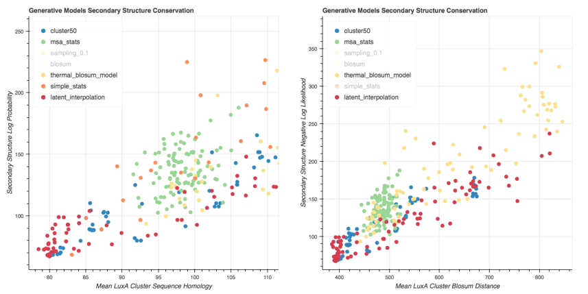> Scatter Plot of Variants generated with the ProtCNN (latent interpolation) and the baseline models. The Negative Log Likelihood is used to assess the secondary structure conservation. Sequence metrics: $d_{mean}$ (Left) and $d_{blosum}$ (Right).

We can see that the Msa Stats Model provides variants that have a worse Secondary Structure Score than the Cluster on average. The performance of the Thermal Blosum Model and the ProtCNN model are roughly the same for the $d_{mean}$ distance metric, and the Thermal Blosum Model is slightly worse with the $d_{blosum}$ distance metric because it tends to select mutations that account for a smaller Blosum Distance.

Here is the same scatter plot using the $d_{min}$ distance:

The Cluster Variants have a Min Cluster Sequence Alignment Distance of 0 as expected. For more than 20 mutations, the Simple Stats model provides a Secondary Structure NLL always too high compared to the cluster; The ProtCNN model seems to be quite good for this metric, since it generates a lot of variants that have between 0 and 80 mutations and that have a low secondary structure score.

Limitations

• Although the dataset of Luciferase share a lot of secondary structure properties, computations made with PSIPRED show a lot of variance in those secondary structures. It could be that they truly have different secondary structures and in that case the model could encode secondary structure information in the latent space, making a sampling approach irrelevant for secondary structure conservation. This is however unlikely.
• The PSIPRED predictions are noisy and from the results above, it is difficult to assess if a generative model is really better than the other. We tried to reduce this noise with the Negative Log Likelihood metrics, but it is hard to know if this is enough. At least, it shows that random mutations spoil the Secondary Structure of the protein.
• Even if our model scores well according to this metric, it doesn't mean that the tertiary structure of a synthetized variant will be the same as in the LuxA cluster and that this variant will be functional.

Contact Map

When the protein acquires its native folding, some amino-acids are in contact and therefore interact strongly with one another. This pattern is reflected in the covariation of sites in the sequence of the protein. Given an alignment of multiple sequences, it has been proposed to consider correlations between sites as indicators of contact in the native folding.

Two positions in the sequence that are in contact are likely to show co-evolution across a protein family.

However, correlations might appear from biased sampling as well as from indirect coupling between sites. That is why looking at the correlations only give poor results. More recent studies take these effects into account, giving relatively accurate contact prediction tools, including Direct Coupling Analysis ^[35], Pseudo Likelihood Methods ^[36] and even Deep-Neural network based methods ^[37].
These methods output what is called a contact map, which is a two-dimensional representation of the three-dimensional protein structure showing which residues are in contact for a specified distance cutoff. The level of gray shows the probability of two residues being in contact.

> The example above shows a contact (yellow dashed line) between two strands of a protein structure, on the right. The same contact is also shown on the contact map as a yellow-filled circle. Notice the rainbow color on both the structure and contact map: the blue region is in contact with the green region.

We submitted an alignment of our Luciferase-Like dataset to GREMLIN, an online software for the computation of contact maps from multiple sequence alignment; The result is shown below. For comparison, we provide a contact map for the LuxA protein in the dataset, computed from physical measures.

Left: Contact Map calculated by Gremlin with the multiple sequence alignment. Right: Contact Map of LuxA determined through X-ray crystallography.

A qualitative metric for our model is to test whether the generated sequences have the desired residues correlations, which should be seen in the contact map calculated from their alignment. One approach is to reconstruct proteins from the dataset, align them, and compute the contact map through residues correlations. This method is however biased, because the good overall reconstruction accuracy will result in the reconstructed sequences having correlations similar to the input dataset.

We therefore generate variants of a single protein LuxA. The generated variants should theoretically reflect the correlation of the dataset since residues in contact could not be changed independently without altering the structure of the protein.

To this purpose, we sample the latent space around the latent representation of LuxA, according to two methods: gaussian sampling and ellipsoid sampling. The gaussian sampling consists in adding a gaussian noise to the latent representation of LuxA.
The ellipsoid sampling tries to take into account the latent structure of LuxA's cluster. It considers that the directions in which there are the most variance in this latent structure are interesting directions to explore when sampling the latent space.
The detailed algorithm is:

• Compute the latent representation of each protein in LuxA's cluster50, which is the latent cluster.
  Compute a PCA with $n$ components of the latent cluster.
  The PCA gives n vectors $z_1$, ... $z_n$, where we consider that the norm of each vector is equal to the standard deviation of the latent cluster according to the vector's direction.
• compute $z_{mean}$ the mean point of the latent cluster
• Sample the distribution ${z_{mean} + \sum_i^n r_i z_i}$ where $r_i \sim \mathscr{N}(0,1)$

We generated 10000 samples with the two methods, which give the following results:

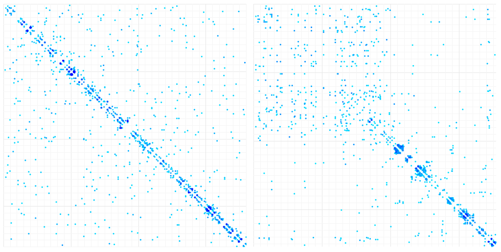
Contact Map of aligned variants of a single protein (LuxA). Left: Gaussian sampling. Right: Ellipsoid Sampling

For the gaussian methods, the results are disappointing: Apart from short-range correlations, there is too much noise in the correlation data to display contact patterns. The ellipsoid pattern are a little more convincing and reflect mostly long-range interaction in the first part of the protein sequence and short-range interactions in the second half of the sequence, which are less homogeneous than in the gaussian sampling.

It could mean than the generated sequences do not reproduce the correlation patterns of the input dataset. This correlations are however hidden in a multiple sequence alignment and are probably too hard to find for our model. It could also be that the correlation signal in the generated variants is mixed with a lot of side correlations which spoils the contact map analysis.

This method might hold some promises but is yet far from producing the expected results.

Experimental Results

Finally, we sought to experimentally validate the ability of ProtCNN to generate functional protein variants. To this end we generated variants of the luxA gene from Photorhabdus luminescens. Protein variants were generated by ProtCNN by randomly sampling the latent space around the representation of luxA. A set of 23 variants more or less distant from the LuxA primary sequence were chosen spanning between 11 and 34 amino acid differences. The variants are chosen so that they have a minimum pairwise distance of 10 and that they are no closer to another protein of the training dataset. DNA sequences encoding these proteins were synthesized and introduced in E. Coli strains, while ensuring that they would all be expressed at the same level. Luminescence could be measured for 17/23 (74%) of the variants, with the most distant variants still producing light carrying 27 mutations.

However, these experimental results are to be taken carefully because of many reasons :

• Dataset Structure: the proportion of luciferase-like proteins in the dataset that effectively produce light is unknown, so the latent space could encode high-level features that do not reflect the light-emitting property.
• Absence of Control Model: It could be that randomly mutating 5% of positions in a protein still allows to conserve the light-emitting property. This is however very unlikely and a mutation rate of 5% is often believed to remove the chemical property of a protein. This hypothesis would still need to be tested however and switching close amino-acids with respect to the blosum matrix could perhaps allow to generate functional variants with a mutation rate as high as 5%.
• Cost of DNA synthetizing: Since synthetizing DNA variants is very expensive, this experiment can be conducted with only a few variants, which explains why no control model has been used.

Conclusion

Measuring the quality of generative models is quite hard because computing the true distribution of the input dataset is generally intractable. Lattice Proteins, which are highly simplified models of proteins, offer a nice framework in which generative models can be evaluated through a fitness metric that reflects the folding quality of a generated protein inside a given structure. Basic Variational Auto Encoders outperform sequence alignment-based methods and bio-inspired methods according to this fitness metric. However, a database of lattice proteins is artificially created through Monte Carlo sampling, and real protein databases are biased due to natural evolution.

Training a Conditional VAE with an autoregressive decoder on a dataset of luciferase-like proteins provides a compressed latent representation of those proteins, allowing to perform arithmetic operations on the latent space. This model is able to understand interchangeability properties between amino-acids and to modify high-level features of a protein with conditioning. We used a metric to evaluate whether ProtCNN was able to generate distant variants of a protein with a consistent secondary structure, compared to other statistical and blosum-based methods : The model showed good performance that ought to be taken carefully due to the inherent difficulty of computing the secondary structure of a protein. We also tried to check whether sites correlations in generated variants could reveal contacts in a protein, similarly to what is done with sequence alignment-based contact calculation methods, with no convincing results.

Overall, it is a highly challenging problem to assess whether a generative model produces functional variants of a protein with computational methods. Only experimental methods can really demonstrate functionality but the high cost of DNA synthetizing makes this approach impossible for the moment. However, the fact that our model scores relatively well on very different metrics is a sign that neural generative models offer promising tools to explore the protein space.

Future Work

In the current model, random sampling of the latent space frequently yielded invalid proteins. Strategies to solve this problem have been proposed, in particular Adversarial Auto Encoders, that add a discriminator network to an autoencoder ^{[28:1] [38]}. The discriminator is trained to differentiate randomly sampled points in the latent space from the projection of actual data. The encoder is trained to fool this discriminator, thus forcing projections to occupy the while latent space and ensuring all points of the latent space can be decoded into valid samples.

Generative Adversarial Networks ^{[39] [40]} are a kind a generative model that generates realistic samples from noise, through a generator network trained to fool a discriminator network. While it remains a challenge to apply GANs to discrete data, recent studies proposed a strategy for that purpose ^[41], that could be worth investigating.

Future work may focus on exploring the latent representation, scaling the model to bigger datasets, and provide more control over the generated sequences. Providing Structural information to the model might also be an interesting idea to generate variants with a fixed secondary structure.

---

1. Packer MS, Liu DR. Methods for the directed evolution of proteins. Nat Rev Genet. 2015;16: 379–394. ↩︎

2. Huang P-S, Boyken SE, Baker D. The coming of age of de novo protein design. Nature. 2016;537: 320–327. ↩︎

3. Gainza P, Nisonoff HM, Donald BR. Algorithms for protein design. Curr Opin Struct Biol. 2016;39: 16–26. ↩︎

4. Gómez-Bombarelli R, Duvenaud D, Hernández-Lobato JM, Aguilera-Iparraguirre J, Hirzel TD, Adams RP, et al. Automatic chemical design using a data-driven continuous representation of molecules, 2016. Available: http://arxiv.org/abs/1610.02415 ↩︎

5. Segler MHS, Kogej T, Tyrchan C, Waller MP. Generating Focussed Molecule Libraries for Drug Discovery with Recurrent Neural Networks, 2017. Available: http://arxiv.org/abs/1701.01329 ↩︎

6. Olivecrona M, Blaschke T, Engkvist O, Chen H. Molecular De Novo Design through Deep Reinforcement Learning, 2017. Available: http://arxiv.org/abs/1704.07555 ↩︎

7. Biswas S., Kuznetsov G., Ogden P., Conway N., Adams R., Church G., Toward machine-guided design of proteins, bioRxiv 337154; Available: https://doi.org/10.1101/337154 ↩︎

8. Kingma DP, Welling M., Auto-Encoding Variational Bayes, 2013. Available: http://arxiv.org/abs/1312.6114v10 ↩︎ ↩︎

9. Rezende DJ, Mohamed S, Wierstra D. Stochastic Backpropagation and Approximate Inference in Deep Generative Models, 2014. Available: http://arxiv.org/abs/1401.4082 ↩︎

10. Walker J, Doersch C, Gupta A, Hebert M., An Uncertain Future: Forecasting from Static Images using Variational Autoencoders, 2016. Available: http://arxiv.org/abs/1606.07873 ↩︎

11. Kulkarni TD, Whitney W, Kohli P, Tenenbaum JB. Deep Convolutional Inverse Graphics Network, 2015. Available: http://arxiv.org/abs/1503.03167 ↩︎

12. Dosovitskiy A, Springenberg JT, Tatarchenko M, Brox T. Learning to Generate Chairs, Tables and Cars with Convolutional Networks, 2014. Available: http://arxiv.org/abs/1411.5928 ↩︎

13. Tim Salimans, Ian Goodfellow, Wojciech Zaremba, Vicki Cheung, Alec Radford, Xi Chen, Improved Techniques for Training GANs, 2016, Available : http://arxiv.org/abs/1606.03498 ↩︎

14. Kristina Preuer, Philipp Renz, Thomas Unterthiner, Sepp Hochreiter, Günter Klambauer. Fréchet ChemblNet Distance: A metric for generative models for molecules, 2018, Available: http://arxiv.org/abs/1803.09518 ↩︎

15. Henikoff, S., & Henikoff, J. G. (1992). Amino acid substitution matrices from protein blocks. Proceedings of the National Academy of Sciences of the United States of America, 89(22), 10915–10919. Available : https://www.ncbi.nlm.nih.gov/pmc/articles/PMC50453/ ↩︎

16. Jacquin, H., Gilson, A., Shakhnovich, E., Cocco, S., & Monasson, R. (2016). Benchmarking Inverse Statistical Approaches for Protein Structure and Design with Exactly Solvable Models. PLoS Computational Biology, 12(5), Available : http://doi.org/10.1371/journal.pcbi.1004889 ↩︎ ↩︎ ↩︎

17. Jérôme Tubiana, Simona Cocco, Rémi Monasson,
    Learning protein constitutive motifs from sequence data, 2018, Available: https://arxiv.org/abs/1803.08718 ↩︎

18. Miyazawa A, Jernigan R. Estimation of effective interresidue contact energies from protein crystal structures: quasi-chemical approximation. Macromolecules. 1985;18:534 Available: http://dx.doi.org/10.1021/ma00145a039 ↩︎

19. Berezovsky IN, Zeldovich KB, Shakhnovich E. Positive and Negative Design in Stability and Thermal Adaptation of Natural Proteins. PLoS Comput Biol. 2007. 03;3(3):e52 10.1371/journal.pcbi.0030052 Available: http://dx.doi.org/10.1371/journal.pcbi.0030052) ↩︎

20. Gulrajani I, Kumar K, Ahmed F, Taiga AA, Visin F, Vazquez D, et al. PixelVAE: A Latent Variable Model for Natural Images, 2016. Available: http://arxiv.org/abs/1611.05013 ↩︎ ↩︎

21. Hochreiter S, Schmidhuber J. Long short-term memory. Neural Comput. 1997;9: 1735–1780. ↩︎

22. Chung J, Gulcehre C, Cho K, Bengio Y. Empirical Evaluation of Gated Recurrent Neural Networks on Sequence Modeling, 2014. Available: http://arxiv.org/abs/1412.3555 ↩︎

23. Shaojie Bai, J. Zico Kolter, Vladlen Koltun, An Empirical Evaluation of Generic Convolutional and Recurrent Networks for Sequence Modeling, 2018, Available: http://arxiv.org/abs/1803.01271 ↩︎

24. van den Oord A, Dieleman S, Zen H, Simonyan K, Vinyals O, Graves A, et al. WaveNet: A Generative Model for Raw Audio, 2016. Available: http://arxiv.org/abs/1609.03499 ↩︎ ↩︎

25. van den Oord A, Kalchbrenner N, Vinyals O, Espeholt L, Graves A, Kavukcuoglu K. Conditional Image Generation with PixelCNN Decoders, 2016. Available: http://arxiv.org/abs/1606.05328 ↩︎

26. van den Oord A, Kalchbrenner N, Kavukcuoglu K. Pixel Recurrent Neural Networks, 2016. Available: http://arxiv.org/abs/1601.06759 ↩︎

27. Gehring J, Auli M, Grangier D, Yarats D, Dauphin YN. Convolutional Sequence to Sequence Learning, 2017. Available: http://arxiv.org/abs/1705.03122 ↩︎

28. Makhzani A, Frey B. PixelGAN Autoencoders, 2017. Available: http://arxiv.org/abs/1706.00531 ↩︎ ↩︎

29. Rice P, Longden I, Bleasby A. EMBOSS: the European Molecular Biology Open Software Suite. Trends Genet. 2000;16: 276–277. ↩︎

30. Kingma DP, Ba J. Adam: A Method for Stochastic Optimization, 2014. Available: http://arxiv.org/abs/1412.6980 ↩︎ ↩︎

31. Sergey Ioffe, Christian Szegedy, Batch Normalization: Accelerating Deep Network Training by Reducing Internal Covariate Shift, 2015. Available: http://arxiv.org/abs/1502.03167 ↩︎

32. He K, Zhang X, Ren S, Sun J. Delving Deep into Rectifiers: Surpassing Human-Level Performance on ImageNet Classification, 2015. Available: http://arxiv.org/abs/1502.01852 ↩︎

33. He H, Garcia EA. Learning from Imbalanced Data. IEEE Trans Knowl Data Eng. 2009;21: 1263–1284. ↩︎

34. Jones DT. Protein secondary structure prediction based on position-specific scoring matrices. J Mol Biol. 1999;292: 195–202. ↩︎

35. Faruck Morcos, Andrea Pagnani, Bryan Lunt, Arianna Bertolino, Debora S. Marks, Chris Sander, Riccardo Zecchina, José N. Onuchic, Terence Hwa, and Martin Weigt, Direct-coupling analysis of residue coevolution captures native contacts across many protein families, 2011. Available: https://doi.org/10.1073/pnas.1111471108 ↩︎

36. Magnus Ekeberg, Tuomo Hartonen, Erik Aurell, Fast pseudolikelihood maximization for direct-coupling analysis of protein structure from many homologous amino-acid sequences, 2014. Available: https://arxiv.org/abs/1401.4832 ↩︎

37. David T Jones, Shaun M Kandathil, High precision in protein contact prediction using fully convolutional neural networks and minimal sequence features, 2018, Available: https://doi.org/10.1093/bioinformatics/bty341 ↩︎

38. Makhzani A, Shlens J, Jaitly N, Goodfellow I, Frey B. Adversarial Autoencoders, 2015. Available: http://arxiv.org/abs/1511.05644 ↩︎

39. Goodfellow IJ, Pouget-Abadie J, Mirza M, Xu B, Warde-Farley D, Ozair S, et al. Generative Adversarial Networks, 2014. Available: http://arxiv.org/abs/1406.2661 ↩︎

40. Goodfellow I. NIPS 2016 Tutorial: Generative Adversarial Networks, 2016. Available: http://arxiv.org/abs/1701.00160 ↩︎

41. Devon Hjelm R, Jacob AP, Che T, Cho K, Bengio Y. Boundary-Seeking Generative Adversarial Networks, 2017. Available: http://arxiv.org/abs/1702.08431 ↩︎