Robust Frank-Wolfe Algorithm for Minimum Enclosing Bregman Balls

This post gathers theoretical convergence & complexity results on the Frank-Wolfe algorithm extended to Bregman divergences (instead of euclidian distance) and made robust to outliers. It is the result of a collaboration with Amaury Sabran, supervised by Pr Frank Nielsen (LIX).

We propose a robust algorithm to approximate the slack minimum enclosing ball problem for a broad class of distance functions called Bregman Divergences.
The slack minimum enclosing ball problem is a convex relaxation of the minimum enclosing ball problem that allows outliers. Bregman divergences include not only the traditional (squared) Euclidean distance but also various divergence measures based on entropic functions. We apply this algorithm to the case of Euclidean MEB, MEB in a Reproducing Kernel Hilbert Space and MEB on the probability simplex with KL-divergences.

Introduction

The minimum enclosing ball of a set of points is the smallest ball that contains all these points. Such balls are used in clustering ^[1] and classification ^[2] problems.

The Standard Minimum Enclosing Ball Problem

For the standard minimum enclosing ball problem, we consider an euclidean vector space $(E, <\cdot,\cdot>)$ and points $(z_1, \cdots, z_n)$ in $E$. The aim is to find the ball $B(c, R)$ with minimum radius that contains all the points. This problem can be described as the following convex optimization problem :

$\operatorname{argmin}_{c \in E} R^2$

$s.t. \quad \Vert c-z_i \Vert^2 \leq R^2,\quad i=1..n$
The radius of the enclosing ball is $R = \max_i \Vert c-z_i \Vert$.

The Slack-Bregman MEB Problem

We generalize this euclidian problem to the case where the distance is derived from a Bregman divergence. Bregman divergences include the standard Euclidean squared distance, the squared Mahalanobis distance and entropy-based distances such as the Kullback–Leibler divergence.

In addition, we generalize the hard-ball problem to slack-balls, i.e enclosing balls allowing outliers. To do so, we add slack variables in the optimization problem that penalize the presence of outliers. We control the amount of outliers with a slack parameter $C$. For $C\geq 1$, we retrieve the hard enclosing ball problem.

The slack Bregman MEB problem ($C$-SMEBB problem) is the following :
$\min_{R,\xi,\theta_c} R + C\sum_{1\leq i \leq n}{\xi_i}$

$s.t \quad A_{F,F^*}(\theta_i : \nabla f(\theta_c)) \leq R + \xi_i ,1 \leq i \leq n,$

$\xi \geq 0$

where $A_{F,F^*}$ is the canonical Bregman divergence defined in a following section.

Definition. A $C$-Slack Minimum Enclosing Bregman Ball of $P$, or $C$-SMEBB of $P$, is an optimal solution $(\theta^*, R^*)$ to this optimization problem.

Related work

The Frank-Wolfe algorithm

The first algorithm to iteratively solve a quadratic program on a simplex has been described by Frank and Wolfe in 1956 ^[3]. The algorithm computes the gradient of the function to minimize, and then makes a small step in the direction in which the gradient is the smallest. The convergence rate of this algorithm is $\Theta(1/k)$, where $k$ is the number of steps. It means that the gap between the algorithm value and the optimal value at step $k$ is smaller than $C/k$ for some constant $C$.
This algorithm could be directly applied to the Minimum Enclosing Ball problem. At each step of the algorithm, the gradient is smallest in the direction of the farthest point from the approximate ball center. This means that the center should make a small step toward the furthest point in the dataset. The objective function of this minization problem is not continuously differentiable; however, geometrical methods in ^[4] showed a similar convergence rate to the general Frank-Wolfe algorithm.

There exists many variants of the Frank-Wolfe algorithm, notably with the ideas of "line search" instead of fixed-size steps, away-steps, and partial computation of the gradient to speed up the algorithm. In this paper, we focused on the original definition of the Frank-Wolfe algorithm, but of course many variants could be adapted to the Bregman divergence-generalization.

Core-sets

Given a set of points $P \subset \mathbb{R}^d$, and $\epsilon>0$, an $\epsilon$-core-set $S$ is a subset of $P$ with the property that the smallest ball containing $S$ is within $\epsilon$ of the smallest ball containing $P$. That is if the smallest ball that contains $S$ is expanded by $1+\epsilon$, then the expanded ball contains $P$.
Core-sets are related to the minimum enclosing ball problem because it is easier to compute an enclosing ball on a smaller subset of $P$.

In ^[4:1], the algorithm to solve the minimum enclosing ball problem is to compute the center as a convex combination of the points in the dataset, and to iteratively add new points to the center representation. It has been shown that after $\frac{1}{\epsilon^2}$ iterations, the center is a convex combination of the points $\theta_1, \cdots, \theta_m$ so that those points are an $\epsilon$-core-set of $P$. In ^[5], it is proven that the optimal size of an $\epsilon$-core-set of any set of point $P$ is $\lceil \frac{1}{\epsilon}\rceil$ and that the bound is tight. This result is remarkable because it does not depend on the number of points in the dataset nor on the dimension of the data.

Therefore, theoretically, in the MEB problem, an $\epsilon$-approximation of the MEB center could be expressed as a convex combination of at most $1/\epsilon$ points. When the dimension d is fixed and finite, the MEB center can always be expressed as a convex combination of at most $d+1$ points.

Our approach

Frank-Wolfe Algorithm for the Slack Bregman MEB problem

Main Result

Let $E$ be a vector space, $<\boldsymbol{\cdot}, \boldsymbol{\cdot}>$ a scalar product over $E$ and $n$ a non-negative integer.
Let $P = \{\theta_1, \theta_2, \cdots, \theta_n\}$ a finite subset of $E$.
Let $F$ be a convex, continuously differentiable function over $T$.
For a function $f$ defined over a convex domain $D$, we define the curvature constant :
$C_f = \sup_{x, s \in D, \gamma \in [0,1], \atop y = x + \gamma (s-x)} \quad \frac{2}{\gamma^2} ( f(x) - f(y) - <y-x, \nabla f(x)>)$

Let $D_F$ be the Bregman divergence associated to $F$ and $A_{F,F^*}$ its canonical divergence as described in the following section.

We note :
$\Delta_n = \{\mathbf{\alpha} \in \mathbb{R}^n : \forall i \in 1..n, 0\leq \alpha_i \leq 1, \sum_i \alpha_i = 1\}$

$C\Delta_n = \{\mathbf{\alpha} \in \mathbb{R}^n : \forall i \in 1..n, 0\leq \alpha_i \leq C, \sum_i \alpha_i = 1\}$

and $(e_i)_{1\leq i\leq n}$ the canonical base of $\Delta_n$.

We define the Slack Bregman Frank-Wolfe algorithm, that output $\theta,R$, the center and radius of the approximate $C$-SMEBB.

• Let $\alpha^{(0)} \in C\Delta_n$

• Let $m = \lceil\frac{1}{C}\rceil$

• For $k = 0...K$ do:

  • $\theta^{(k)}:=\sum{\alpha_i^{(k)} \theta_i}$

  • $\eta^{(k)} := \nabla F (\theta^{(k)})$

  • $D^{(k)} :=(A_{F,F^*}(\theta_i : \eta^{(k)}))_{1\leq i \leq n}$

  • Let $i_1, \cdots , i_m$ be the indices of the $m$ largest entries of D (unsorted) with $i_m$ the index of the $m$-th largest entry.

  • $s^{(k)} :={\sum_{k=1}^{m-1} C e_{i_k}}+ (1-(m-1)\cdot C)e_{i_m}$

  • $R^{(k)} := A_{F,F^*}(\theta_{i_m} : \eta^{(k)})$

  • $gap^{(k)} := <s^{(k)}-\alpha^{(k)},D^{(k)}>$

  • $\alpha^{(k+1)}=(1-\gamma_k)\alpha^{(k)} + \gamma_k s^{(k)} \text{ where }\gamma_k = 2/(k+2)$

• Let $j := \operatorname{argmin}_k gap^{(k)}$

• Let $\theta,R := \theta^{(j)}, R^{(j)}$

Theorem [Couairon, Sabran]. Let $(\theta^*, R^*)$ be a $C$-SMEBB of $P$. Let $(\theta, R)$ be the center and radius of the Bregman ball computed by the following algorithm during $K$ steps.

Then,
$\quad D_F(\theta^*,\theta) \leq \frac{4 C_F}{K+2}$

This algorithm lets us approximate the center of a Slack Bregman Minimum Enclosing ball with a convergence rate of $\Theta(1/k)$.

Background Tools and results

In this post, we will not prove the above theorem, but we will present the tools we used from Bregman geometry and convex optimization.

Bregman Divergence

Let $\chi$ be a compact convex subset of $\mathbb{R^d}$. Let $D_F (\theta_1 : \theta_2)$ denote the Bregman divergence for a smooth strictly-convex real-valued generator $F : \chi \mapsto \mathbb{R}$.
$D_F (\theta_1 : \theta_2) = F(\theta_1)-F(\theta_2)-<\theta_1-\theta_2, \nabla F(\theta_2)>$.

Informally speaking, the Bregman divergence $D_F$ is the tail of the Taylor expansion. $D_F (\cdot : \theta_2)$ can be interpreted as the distance between $F$ and its linear approximation around $\theta_2$ as shown below. Since F is strictly convex, $D_F(\theta_1 :\theta_2) \geq 0$ and $D_F(\theta_1 :\theta_2) = 0$ iff $\theta_1 = \theta_2$.

Visualizing the Bregman divergence

Consider the dual convex conjugate of $F$, $F^*(\eta) = \sup_{\theta}{<\theta, \eta>- F(\theta)}$. We have $D_F(\theta_1:\theta_2)= D_{F^*}(\eta_2 :\eta_1)$ with $\eta = \nabla F (\theta)$. (and $\theta = \nabla F^*(\eta)$ so that $\nabla F \circ \nabla F^* =$ id). Define the canonical divergence $A_{F,F^*}(\theta_1 : \eta_2) = F(\theta_1) + F^*(\eta_2) -<\theta_1, \eta_2>$.

We have $D_F(\theta_1 :\theta_2) = D_{F^*}(\eta_2 : \eta_1) = A_{F,F^*}(\theta_1 : \eta_2)$

$A_{F,F^*}$ is convex in its first and second arguments.

We define a right-centered Bregman ball $ball_F(\eta_c,r) = \{\theta \in \chi | A_{F,F^*}(\theta,\eta_c) \leq r\}$.

Given a finite set of points $P=\{\theta_1,...\theta_n\} \subset \chi$, the right-centered Minimum Enclosing Bregman Ball (rMEBB) is defined as the unique minimizer of $\min_{\eta_c}\max_{1\leq i \leq n}{A_{F,F^*}(\theta_i,\eta_c)}$

Wolfe Duality

Consider a general optimization problem:
$\min_x f(x)$

$s.t. \quad g_i(x) \leq 0, i=1..m$

The Lagrangian Dual problem is
$\max_{u} \quad \inf_x \quad f(x) + \sum_j^m u_j g_j(x)$

$s.t. \quad u_j \geq 0, j=1..m$

Provided that the functions $f$, $g_1$, ... $g_m$ are convex and differentiable and that a solution exists, the infimum occurs when the gradient is equal to 0. The Wolfe Dual problem uses the KKT conditions as a constraint. The problem is therefore
$\max_{x, u} f(x) + \sum_{j=1}^m u_j g_j(x)$

$s.t. \quad \nabla f(x) + \sum_{j=1}^m u_j \nabla g_j(x) = 0$

$u_j \geq 0, j=1..m$

Let us write the Wolfe dual to the SMEBB optimization problem.
By identification, we have
$f(\eta, R, \xi) = R + C\sum_{1\leq i \leq n} \xi_i$

$g_i(\theta_i, \eta_c) = A_{F,F^*}(\theta_i : \eta_c) - R - \xi_i, \quad i=1..n$

$g_i(\xi) = - \xi_i, \quad i=(n+1)...2n$

$f, g_1, ..., g_{2n}$ are convex and differentiable with respect to the variables $R$, $\eta_c$, $\xi$. Therefore the Wolfe dual is

$\max_{\eta, R, \xi, \alpha, \mu} R + \sum_{1\leq i \leq n} \alpha_i (A_{F,F^*}(\theta_i : \eta_c) - R - \xi_i) + \sum_{1\leq i \leq n} (C-\mu_i) \xi_i$

$s.t. \alpha_i \geq 0, \mu_i \geq 0 , \alpha_i + \mu_i = C \quad i = 1..n$

$\eta = \nabla F (\sum_{1\leq i \leq n} \alpha_i \theta_i), \quad \sum_{1\leq i \leq n} \alpha_i= 1$

From now on, we define the following maps:
$\theta(\alpha) = \sum_{1\leq i \leq n} \alpha_i \theta_i \quad \text{and} \quad \eta(\alpha) = \nabla F (\theta(\alpha))$

The Wolfe dual of the SMEBB problem can be simplified as
$\max_{\alpha \in C\Delta_n} \sum_{1\leq i \leq n} \alpha_i A_{F,F^*}(\theta_i : \eta(\alpha))$

We define the Wolfe dual function over $C\Delta_n$:
$f(\alpha) = \sum_{1\leq i \leq n} \alpha_i A_{F,F^*}(\theta_i : \eta(\alpha))$

We can also write
$f(\alpha) = \sum_{1\leq i \leq n}{\alpha_i F(\theta_i)}-F(\theta(\alpha))$

this dual function is concave over $C\Delta_n$.

Jaggi's theorem

The Slack Bregman Frank-Wolfe algorithm is the Frank-Wolfe optimization algorithm applied with the Wolfe dual problem of the SMEBB problem. The convergence theorem is from Jaggi (2008) ^[6].

Theorem [Jaggi, 2008]. Let $f$ be a convex, continuously differentiable function, and $D$ a compact convex subset of any vector space.;
Let $x^* = \min_{x \in D} f(x)$ and $C_f$ be the curvature constant of $f$;
Let $g$ be the duality gap:
$g(x) = \max_{s \in D} \quad <x-s, \nabla f(x)>$

Consider a sequence $(x^{(k)})$ computed by the Frank-Wolfe algorithm :

• Let $x^{(0)} \in D$
• For $k = 0...K$ do:
  • Compute $s:= \operatorname{argmin}_{s \in D}{<s, \nabla f(x^{(k)})>}$
  • Update $x^{(k+1)} = (1-\gamma_k) x^{(k)} + \gamma s$ where $\gamma_k = 2/(k+2)$

Then,
$\min_{1\leq k\leq K} g(x^{(k)}) \leq \frac{4 C_f}{K+2}$

The duality gap is an upper bound of the difference between the values of the primal and dual functions.

Proof of the theorem

We only provide a sketch of the proof: First, we show that our algorithm is the Frank-Wolfe algorithm applied to $-f$ where $f$ is the dual function of the $C$-SMEBB problem. We then analyze to duality gap and show that $gap^{(k)} \geq D_F(\theta^*, \theta^{(k)})$.

Therefore,
$D_F(\theta^*,\theta) \leq gap^{(j)} \leq \frac{4 C_F}{K+2}$

Applications

The Frank-Wolfe algorithm lets us approximate the optimal solution to the SMEBB problem.

Definition. An $(\epsilon, C)$ slack Bregman MEB of a set of points $\theta_1, \cdots, \theta_n$ is a couple $(\theta, R)$ such that if $\theta^*$ is an optimal solution to the slack Bregman Meb problem, then
$D_F(\theta^*, \theta) \leq \epsilon$

With this definition, we have the following lemma:
Lemma. The number of iterations needed to compute a $(\epsilon, C)$ slack Bregman MEB of a set of points is $\Theta(C_F/\epsilon)$.

Slack Minimum Enclosing Ball with the Euclidean Distance

In this section, $P = \{\theta_1, \cdots, \theta_n\}$ are points in a vector space $E$ of finite dimension $d$. We consider the euclidean scalar product on $E$, which corresponds to the Bregman divergence $D_F$ associated to the generator $F(\theta) = \theta^T\theta/2$.

The optimization problem is therefore the Minimum enclosing ball problem with outliers:

$\min_{c, R, \xi} R + C\sum_{1\leq i \leq n}{\xi_i}$

$s.t. \quad \Vert c-\theta_i \Vert^2 \leq R + \xi_i ,\quad 1 \leq i \leq n$ $\xi \geq 0$

Theorem. The Slack Bregman Frank-Wolfe algorithm computes a $(\epsilon, C)$-SMEBB of $\mathbf{Z}$ in time $\Theta(nd \Delta /\epsilon)$. where $\Delta = diam(\mathbf{Z})^2$.

Proof. We first notice that for this Bregman divergence, $C_F = diam(\mathbf{Z})^2 = \max_{z,z'} \Vert z-z' \Vert^2$.
With the previous lemma, we have shown that after $\Theta(C_F/\epsilon)$ iterations, the algorithm returns a $(\epsilon, C)$-SMEBB of $P$. Therefore one only need to show that each iteration can be computed in time $\Theta(nd)$.
With $F(z) = z^Tz/2$, we have $\nabla F = Id$ and
$A_{F,F^*}(\theta_a: \eta_b) = \frac{\Vert \theta_a-\theta_b \Vert^2}{2}$

For each iteration, we have $\theta^{(k)} = \sum_{1 \leq i \leq n} \alpha_i^{(k)} \theta_i$ computed in time $\Theta(nd)$, $\theta^{(k)} = \eta^{(k)}$ and $D^{(k)}_i = \frac{ \Vert \theta_i-\theta^{(k)} \Vert ^2}{2}$. Therefore computing each of the $n$ coordinates of $D^{(k)}$ takes time $\Theta(d)$.
Computing the $m$-th largest entries of D takes time $\Theta(n)$ with the introselect algorithm and the remaining operations are all computed in time $\Theta(nd)$, hence the execution time of the algorithm is $\Theta(nd/\epsilon)$.

Our definition of a $(\epsilon, C)$-SMEBB is not the same that the standard euclidian MEB approximation. Usually, a ball $B(c, R)$ is an $(1+\epsilon)$-approximation of the minimum enclosing ball $B(c^*, R^*)$ if $B(c^*,R^*) \subset B(c,(1+\epsilon)R)$.A sufficient condition for $B(c, R)$ to be an $(1+\epsilon)$ approximation of the MEB is $\Vert c-c^* \Vert<\epsilon R^*$. With this definition, the number of iteration needed is $\Theta(1/\epsilon^2)$ and therefore the total execution time is $\Theta(nd/\epsilon^2)$.

Kernelized Slack MEB

In real life, the data is not linearly separable, and euclidian enclosing balls do not reflect the geometry of a dataset. That is why it is interesting to map the data into a feature space through a kernel and to consider enclosing balls in this feature space.

In this section, $\mathbb{Z} = \{z_1, \cdots, z_n\}$ are points in a vector space $E$ of finite dimension $d$. We consider a mapping $\phi$ of $\mathbb{Z}$ into an unknown feature space $F$ such as
$\forall (z,z') \in \mathbb{Z}^2, <\phi(z), \phi(z')> = k(z, z')$
where k is a definite positive kernel, which means that
$\forall c \in \mathbb{R}^n, \sum_{1 \leq i,j \leq n} c_i c_j k(z_i,z_j) \geq 0$
For instance, we could use the gaussian kernel:
$k(z, z') = exp(-q\Vert z-z' \Vert^2)$.

We define $P = \{\theta_1, \cdots, \theta_n\} = \{\phi(z_1), \cdots, \phi(z_n)\}$. The representation of points in $E$ is implicit, which means that the center $c$ of the SMEBB is described as a convex combination of $\{\theta_1, \cdots, \theta_n\}$: $c = \sum_{\alpha \in C\Delta_n} \alpha_i \theta_i$.

Let $G$ be the Graham matrix of P, such that $G_{i,j} = <\theta_i, \theta_j> = k(z_i, z_j)$.

This scalar product corresponds to the Bregman divergence
$D_F$ associated to the generator
$F(\sum_{1 \leq i \leq n} \alpha_i z_i) = \alpha^TG\alpha/2 = \frac{1}{2} \sum_{1\leq i,j \leq n} \alpha_i \alpha_j G_{i,j} \quad \text{for} \quad \alpha \in \Delta_n$

Theorem. The Slack Bregman Frank-Wolfe algorithm computes a $(\epsilon,C)$-SMEBB of $\mathbb{Z}$ in time $\Theta(n \Delta /C\epsilon)$. where $\Delta = diam(\phi(\mathbf{Z}))^2$.

Proof. Since $C_F = \Delta$, the algorithm returns a $(\epsilon, C)$-SMEBB of $P$ in $\Theta(\Delta/\epsilon)$. We only need to show that each iteration can be computed in time $\Theta(n/C)$.
The only difficult point is to show that in the algorithm, is is possible to compute $D^{(k)}$ is time $\Theta(n/C)$. We have
$D^{(k)}_i = (e_i - \alpha^{(k)})^TG(e_i - \alpha^{(k)})$

Since adding a constant term to $D^{(k)}$ does not change the computation of $s^{(k)}$ and $gap^{(k)}$, we can consider
$D^{(k)} = diag(G) - 2 G\alpha^{(k)}$

$D^{(k+1)} = D^{(k)} + 2 G(\alpha^{(k+1)} - \alpha^{(k)})$
The update rule of $\alpha^{(k)}$ shows that the vector $\alpha^{(k+1)} - \alpha^{(k)}$ has at most $1/C$ non-empty entries. Therefore the computation of $G(\alpha^{(k+1)} - \alpha^{(k)})$ takes time $\Theta(n/C)$, hence the total running time of $\Theta(n\Delta/C\epsilon)$.

Kullback-Leibler divergence

When working on a dataset that consist in points in the probability simplex, it is more natural to work with the Kullback-Leibler divergence than with the euclidian distance.

Let $P=(p_1,...p_{d+1})$ denote a point of the d-dimensional probability simplex.
For $1\leq i \leq d$, let
$\begin{aligned} \theta(P) &= (log(\frac{p_i}{p_{d+1}}))_{1 \leq i \leq d} \\ \eta(P) &= (p_i)_i = (\frac{e^{\theta_i}}{1+\sum_{k=1 }^d{e^{\theta_k}}})_{1 \leq i \leq d} \\ \end{aligned}$ and $\begin{aligned} F(\theta) &= log(1+ \sum_{j=1}^d e^{\theta_j})\\ F^*(\eta) &= \sum_{i=1}^d{\eta_i log(\eta_i)}+ (1-\sum_k \eta_k) log (1-\sum_k \eta_k) \end{aligned}$

The Kullback-Leibler divergence between two points P and Q of the d-dimensional probability simplex is $KL(P:Q) = D_F(\theta(Q),\theta(P)) = A_{F,F^*}(\theta(Q),\eta(P))$

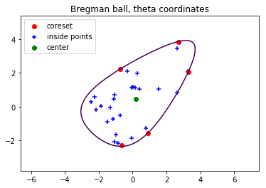
Hard Bregman ball

Bregman balls obtained with the FW Bregman MEB algorithm

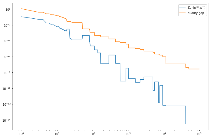
Center convergence rate and duality gap for FW Bregman MEB algorithm

Conclusion

We have considered the Frank-Wolfe algorithm for solving the Minimum Enclosing ball Problem and generalized it to Bregman divergences. We also considered an optimization problem with slack variables, which allow some outliers. We showed that the Frank-Wolfe algorithm can be run within this new framework, and demonstrated a convergence rate of $\Theta(1/k)$ where $k$ is the number of iterations, which is the same as what is proved in the Standard Euclidian MEB problem.

We showed three applications of this result: the standard euclidian slack MEB problem, the kernelized MEB problem where the enclosing ball is computed in a feature space, and MEB on the probability simplex with the Kullback-Leibler divergence.

Further studies may focus on the Nesterov Framework, which is a framework for non-smooth convex optimization. A convergence rate of $\Theta(nd/\sqrt{\epsilon})$ is shown in ^[7].

The MEB problem with outliers on $\mathbb{Z} = \{z_1, \cdots, z_n\}$ can be written as
$\operatorname{argmin}_{c \in E} \quad \Vert c \Vert^2 + \max_{u \in C\Delta_n} (<Ac, u> + <b, u>)$
with $b = (b_1, \cdots, b_n)$ such as $b_i = \Vert z_i \Vert^2$, and $A = -2 (z_1, \cdots, z_n)^T$.

Therefore, one can apply the same method as in the paper for the Slack MEB problem, with $Q_2 = C\Delta_n$ instead of $Q_2 = \Delta_n$. The algorithm developped in this paper could also perhaps be generalized to Bregman divergences.

In another direction, when the approximated center is close enough to the real center, the variable $D^{(k)}$ in the algorithm stays roughly the same, so the computation of the largest entries of $D^{(k)}$ might be easier. It would be a good idea to study which structure should be maintained on the entries of $D^{(k)}$ so that the time complexity of this step decreases over time.

Appendix

Lemma. Let $D = C\Delta_n$ with $1/n \leq C \leq 1$, $m=\lceil\frac{1}{C}\rceil$ and $v \in D$.

The solution to the optimization problem $\operatorname{argmax}_{s \in D}{<s, v>}$ is
$s = \sum_{1 \leq k \leq m-1} Ce_{i_k} + (1-(m-1)C)e_{i_m}$
where $i_1, \cdots, i_m$ are the indices of the $m$-th largest entries of $v$, $i_m$ being the $m$-th largest entry, and is computed in time $\Theta(n)$.

Proof. Let $(I, \{i_m\}, J)$ be a partition of $[\![1;n]\!]$ such that $\Vert J \Vert = \lfloor 1/C \rfloor$ and
$\forall i \in I, \forall j \in J, \quad v_i \leq v_{i_m} \leq v_j$.
This partition can be computed in time $\Theta(n)$, and $J$ is the set of indices of the $m$-th largest entries of $v$.

Let $\lambda = 1 - (m-1)C$, $s = \lambda e_{i_m} + \sum_{j \in J} C e_i$, and $\alpha \in D$.

$\forall i \in I, 0 = s_i \leq \alpha_i$ and $\forall j \in J, 0 \leq \alpha_j \leq s_j$, therefore :
$\begin{aligned} <s - \alpha, v> &= \sum_{i \in I} (s_i - \alpha_i) v_i + (s_{i_m} - \alpha_{i_m}) v_{i_m} + \sum_{j \in J} (s_j-\alpha_j) v_j \\& \geq \sum_{i \in I} (s_i - \alpha_i) v_{i_m} + (s_{i_m} - \alpha_{i_m}) v_{i_m} + \sum_{j \in J} (s_j-\alpha_j) v_{i_m} \\& \geq \sum_{i \in [\![1;n]\!]} (s_i - \alpha_i) v_{i_m} \\&\geq (\sum_{i \in [\![1;n]\!]} s_i - \sum_{i \in [\![1;n]\!]} \alpha_i) v_{i_m} = 0 \end{aligned}$

Therefore,
$\forall \alpha \in D, <s, v> \geq <\alpha, v> \implies s = \operatorname{argmax}_{s \in D}{<s, v>}$

---

1. Ben-Hur, Asa and Horn, David and Siegelmann, Hava T and Vapnik, Vladimir, Support vector clustering, Journal of machine learning research, 2(Dec), 125-137, 2001 ↩︎

2. Tax, David MJ and Duin, Robert PW, Support vector data description, Machine Learning, 54(1):45-66, 2004 ↩︎

3. Frank, Marguerite and Wolfe, Philip, An algorithm for quadratic programming, Naval Res. Logist. Quart., 1956 ↩︎

4. Badoiu, Mihai and Clarkson, Kenneth L, Smaller core-sets for balls, In Proceedings of the fourteenth annual ACM-SIAM symposium on Discrete algorithms, pages 801-802, Society for Industrial and Applied Mathematics, 2003. ↩︎ ↩︎

5. Badoiu, Mihai and Clarkson, Kenneth L, Optimal core-sets for balls, Computational Geometry, 40(1): 14-22, 2008 ↩︎

6. Martin Jaggi, Revisiting Frank-Wolfe: Projection-Free Sparse Convex Optimization, Proceedings of the 30th International Conference on Machine Learning, volume 28 of Proceedings of Machine Learning Research, 2013, Available http://proceedings.mlr.press/v28/jaggi13.pdf. ↩︎

7. Ankan Saha and S. V. N. Vishwanathan, Efficient Approximation Algorithms for Minimum Enclosing Convex Shapes, CoRR, abs/0909.1062, 2009 ↩︎