Kernelized Minimum Enclosing Balls for Machine Learning

In this post, we are going to talk about a very famous problem in computational geometry: the Minimum Enclosing Ball (MEB) problem, which consists in finding the ball that contains a given set of points with minimum radius. We first describe how to compute arbitrarily fine approximations of Minimum
Enclosing Balls in a feature Hilbert space induced by a kernel using the Frank-Wolfe optimization algorithm, and show how to make these balls robust by allowing outliers. We then explain several applications of these robust kernelized MEBs in machine learning by presenting applications to supervised multiclass classification, unsupervised clustering, and deep generative models.

Project in collaboration with Amaury Sabran, supervised by Pr Frank Nielsen (LIX). Video available here.

Minimum Enclosing ball

Definition. The minimum enclosing ball ^[1] of a finite set of points $Z = \{z_1, \cdots, z_m\} \subset \mathbb{R}^d$ is the unique smallest-radius Euclidian ball that fully covers $Z$.

Minimum Enclosing Ball: We can see that as points move in the 2D space, the ball enclosing all the points has always the smallest possible radius.

The MEB can be solved in polynomial time for fixed dimension, but is NP-hard with respect to the dimension $d$ of the vector space. It can be expressed as a convex optimization problem ^[2]:

$\min_{\bold{c}, R} \ R^2$ $s.t. \quad \Vert \bold{z_{i}}-\bold{c}\Vert^2 \leq R^2, \quad i=1..m$

With this formulation, the objective is to minimize the radius $R$ under the constraints that all points lie inside the enclosing ball. It follows that the exact circumcenter can be expressed as a convex weighted combination of the input points $\bold c = \sum_{i=1}^m \alpha_i \bold z_i$ (where $\alpha_i \geq 0$ and $\sum_i \alpha_i = 1$). There are at most $d+1$ points lying on the boundary of the MEB (assuming general position) called the support vectors of the ball ^[3].

This problem can be solved using a Quadratic Programming solver, which does not scale well with high dimensions in practice (say, $d>50$). This is why we resort to approximation algorithms ^{[4] [5] [6]}, and especially the Frank-Wolfe algorithm.

Frank Wolfe Algorithm

In the Frank-Wolfe algorithm ^[7], the center of the minimum enclosing ball is approached by a convex combination of points $\bold{c} = \sum_{i=1}^{m} \alpha_i \bold z_i$, where the $\alpha_i$ are updated at each step of the algorithm. The principle is the following: starting from the center located at an arbitrary point of the dataset, we update the position of the center at step $i$ by moving towards the furthest point with coefficient $1/(i+1)$.

• $\bold c_0 = \bold z_0$
• For $i = 1...N$ do
  • $j = \operatorname{argmax} \Vert \bold c_{i-1} - \bold z_j \Vert$
  • $\bold{c_{i}}= \frac{i}{i+1}\bold c_{i-1} + \frac{1}{i+1} \bold{z_{j}}$

Animation of the Frank Wolfe Algorithm. The convex combination of points converges towards the MEB center.

Badoiu and Clarkson proved that after $1/\epsilon^2$ iterations of the algorithm, the algorithm returns an $\epsilon$-approximation of the ball: $k \geq 1/\epsilon^2 \Rightarrow r_k \leq (1+\epsilon) r^*$, where $r_k$ is the radius of the enclosing ball at step $k$ and $r^*$ the radius of the minimum enclosing ball ^[8]. This is a remarkable result since the quality of the approximation is independent of the space dimension d.

If we want to model the statistical distribution of a dataset with a Minimum Enclosing Ball, we are faced with two problems: considering only euclidian balls is too restrictive and the MEB of a dataset is very sensitive to outliers. That is why we show in the next section how to overcome these problems by building robust, kernelized MEBs.

Kernelized MEB

Few real-life datasets can be well described by an Euclidian Enclosing Ball. We therefore consider a larger class of enclosing balls that are not euclidian, using the kernel trick : Instead of using an euclidian dot product, we use a dot product that comes from a gaussian kernel $k(\bold x, \bold y) = \exp(-\frac{\Vert \bold x-\bold{y}\Vert^2}{2 \sigma^2})$

There is an implicit transformation $\Phi$ associated to this dot product, which maps our data into a feature space. Each point is represented as $\Phi(z_i)$ in this feature space and the scalar product writes $k(\bold x, \bold y) = <\Phi(\bold x), \Phi(\bold y)>$. Since the algorithm only uses dot products between two feature points, we only need the kernel and not the explicit transformation.

We can kernelize the Frank-Wolfe algorithm by maintaining an implicit representation of the feature center, consisting in a convex weighted combination of the feature points:
$\bold{c} = \sum_{i=1}^{m} \alpha_i \Phi(\bold z_i)$

$\alpha_i \geq 0, \quad \sum_i \alpha_i = 1$

The distance between the feature center $\bold c$ and a feature point $\Phi(\bold z)$ is calculated as follows:

$\Vert c - \Phi(\bold z) \Vert ^2 = \sum_{i=1}^m \sum_{j=1}^m \alpha_i \alpha_j k(\bold z_i, \bold z_j) - 2 \sum_{i=1}^m \alpha_i k(\bold z_i, \bold z) + k(\bold z, \bold z)$

If we consider the Graham Matrix $K$ of our input points defined as $K_{i, j} = <\Phi(\bold z_i), \Phi(\bold z_j)> = k(\bold z_i, \bold z_j)$, we can write

$\Vert c - \Phi(\bold z_i) \Vert ^2 = \alpha^T K \alpha - 2\alpha^T K_i + K_{i, i}$

We can reformulate our convex optimization problem as
$\min_{\bold{\alpha}, R} \ R^2$

$s.t. \quad \bold \alpha ^T K \bold \alpha - 2 \bold \alpha ^T K_i +K_{i,i}\leq R^2, \quad i=1..m$

Solving this problem is equivalent to the standard MEB-problem in an unknown Hilbert feature space.

Below, we compute the minimum enclosing ball with a gaussian kernel parameterized by its bandwidth sigma, and draw this ball into the input space. We can see how different values of sigma give different contours for the enclosing ball.

Robust kernelized MEB

The contour given by a minimum enclosing ball is very sensitive to outliers: A single outlier point may corrupt the MEB. We can overcome this issue by introducing a slack parameter $\lambda$ in the optimization problem.
Given a set of points $\bold{Z} = \{z_1, \cdots, z_m\} \subset \mathbb{R}^d$, the slack (or robust) MEB problem is

$\min_{\bold{c}, R} \ \lambda R^2 + \frac{1}{m} \sum_{i=1}^{m} \xi_i$ $s.t. \quad \Vert \bold{z_{i}}-\bold{c}\Vert^2 \leq R^2 + \xi_i, \quad i=1,\cdots, m$ $\xi_i \geq 0, \quad i=1..m$

This parameter can be used to control the number of outliers : the proportion of outliers is bounded by the parameter $\lambda \in \{0, 1\}$.

Controlling the proportion of outliers with $\lambda$.

Applications

Describing data through minimum enclosing balls is useful for many applications. We will focus on multi-class classification with support vector data description, and then talk about segmentation and data augmentation.

Multi-class classification with Support Vector Data Description

Given a labeled training set with $k$ classes, the classification problem consists in classifying new incoming points as belonging to one of theses $k$ classes. When $k=2$, this is called binary classification in machine learning.

Minimum Enclosing Balls give us an accurate description of each class in a dataset, which we can use to classify new data points. Suppose that we have a linearly separable 2D-dataset with two classes, $A$ and $B$. We first compute a minimum enclosing ball for each class. Then, the centers of the enclosing balls induce a Voronoï diagram that we use for classification: new query points are classified as belonging to the class associated to the closest circumcenter.
For two classes, the decision boundary is the radical axis Hyperplane for the power distance.

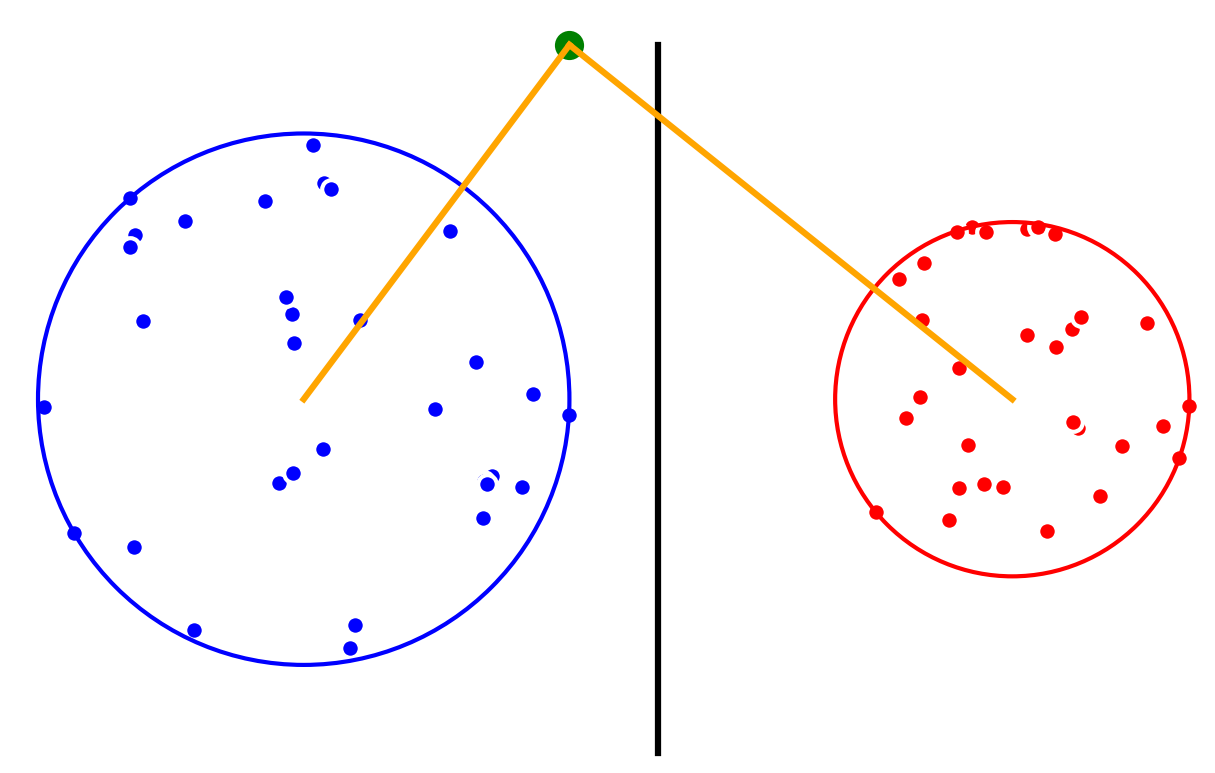
The new point is classified as belonging to class A (blue).

The probablity of belonging to a class is calculated using a score function, the lower the score for class $i$, the higher the probability of belonging to class $i$. In the previous case, the score function is simply the distance to the center.

Alternatively, we can take into account the size of the balls, for instance by using the score function $d(x, c_i)/R_i$ where $B(c_i, R_i)$ is the MEB associated to class $i$.

In that case, the decision boundary is no longer linear :

Colormap associated to the difference between the two score function. Blue line: decision boundary.

But what if our dataset is not linearly separable ? We just use the kernel trick as seen before. We show this on a 2D-dataset with two circles. We use the kernelized Frank-Wolfe algorithm: support vectors are shown in white below.

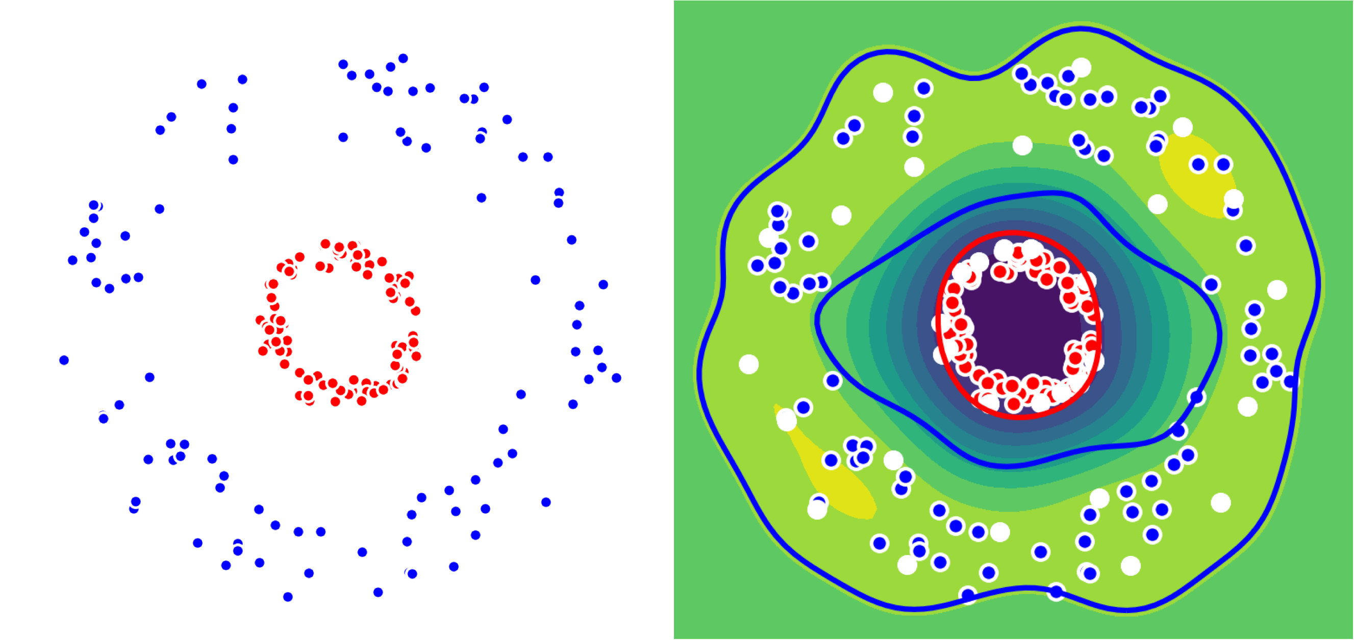
Left: Dataset with two classes (Red, Blue)
Right: Colormap associated to the difference of distances to the two centers.

We used a gaussian kernel to compute the minimum enclosing ball of our two classes. The gaussian kernel is parameterized by its bandwith $\sigma$ on which the classification depends. We show below the decision boundaries associated to different values of the parameter $\sigma$ in the gaussian kernel.

SVDD classification with varying $q = 1/\sqrt \sigma$ for a toy 2D-dataset.

We can see that when $\sigma$ is small enough, there is another boundary that appears : Points very close to the origin will be classified as belonging to the external circle. It means that $\sigma$ must be chosen carefully if we want to use this technique for classification.

Support Vector Clustering

Minimum Enclosing Balls can be used to identify clusters in a dataset. Indeed, the projection of a kernelized MEB onto the input space is not necessarily convex and nor always connected. The Support Vector Clustering (SVC) algorithm ^[9] takes advantage of these connected components to identify clusters in the dataset : each connected component becomes a cluster. To detect whether two points in the data space belong to the same component or not, the straight line segment joining them is discretized (say into 10 steps) and we check whether the interpolated points belong to the MEB or not, in the feature space. If all interpolated feature points belong to the MEB, then the two points are considered to belong to the same connected component.

Below, we show these connected components for different values of the parameter sigma.

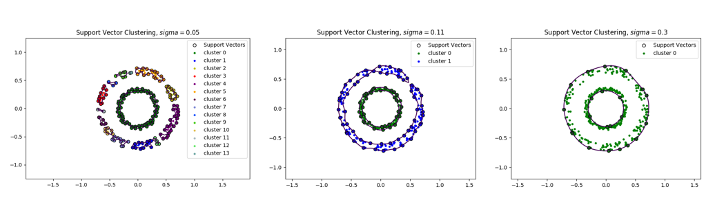
Support Vector Clustering for $\sigma = 0.05$ (Left, 13 clusters), $\sigma = 0.11$ (Center, 2 clusters), $\sigma = 0.3$ (Right, 1 cluster).

We can see that the number of connected components decreases as sigma increases. For a very small value of $\sigma$, each point is found to belong to its own cluster while for a large value of sigma, there is only a single cluster. Thus, the number of clusters is adjusted by choosing an appropriate value of $\sigma$, see ^[9:1].

Geometric Enclosing Networks

The kernelized MEBs can also be used for data augmentation: Suppose that we have a set of points in a metric space (for instance fixed-dimensional images) and that we would like to generate new images that are similar to this training set.

Computing a MEB of the dataset in a feature space gives us an accurate description of the data domain, and the closer a feature point is to the center of the MEB, the more similar this point is from the training set. We therefore need a way to sample this feature space. For that purpose, we consider a neural network that takes random noise as input, and train it to minimize the kernel space distance between the output and the center of the MEB.

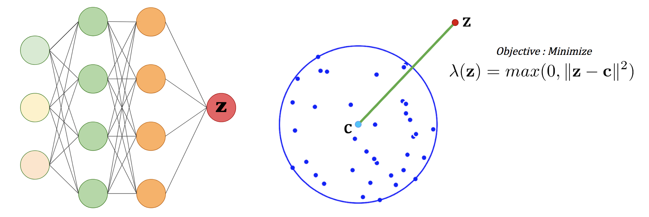
Left: Neural Network.
Right: 2D representation of the optimization objective.

After training, the output of the network will have a small feature distance to the MEB center and thereby will be similar to the images of the training set. This yields a deep generative model ^[6:1].

Conclusion

We have shown how to use the Frank-Wolfe algorithm to compute kernelized minimum enclosing ball for a dataset, and how to take advantage of this powerful representation for multi-class classification, unsupervised clustering and data augmentation.

This post serves as a proof of concept, hence no benchmarking has been done but you can see the methods presented here evaluated with the standard datasets in these papers ^{[9:2] [6:2]}.

---

1. Emo Welzl. Smallest enclosing disks (balls and ellipsoids). New results and new trends in computer science, pages 359–370, 1991. ↩︎

2. Bernd Gärtner and Sven Schönherr. An efficient, exact, and generic quadratic programming solver for geometric optimization. In Proceedings of the sixteenth annual symposium on Computational geometry, pages 110–118. ACM, 2000. ↩︎

3. Bernhard Scholkopf and Alexander J. Smola. Learning with Kernels: Support Vector Machines, Regularization, Optimization, and Beyond. MIT Press, Cambridge, MA, USA, 2001. ↩︎

4. Yaroslav Bulatov, Sachin Jambawalikar, Piyush Kumar, and Saurabh Sethia. Hand recognition using geometric classifiers. Biometric Authentication, pages 1–29, 2004. ↩︎

5. David MJ Tax and Robert PW Duin. Support vector data description. Machine learning, 54(1):45–66, 2004. ↩︎

6. Trung Le, Hung Vu, Tu Dinh Nguyen, and Dinh Phung. Geometric enclosing networks. arXiv preprint arXiv:1708.04733, 2017. ↩︎ ↩︎ ↩︎

7. Martin Jaggi. Revisiting Frank-Wolfe: Projection-free sparse convex optimization. In International Conference on Machine Learning, pages 427–435, 2013. ↩︎

8. Mihai Badoiu and Kenneth L Clarkson. Smaller core-sets for balls. In Proceedings of the fourteenth annual ACM-SIAM symposium on Discrete algorithms, pages 801–802. Society
   for Industrial and Applied Mathematics, 2003. ↩︎

9. Asa Ben-Hur, David Horn, Hava T Siegelmann, and Vladimir Vapnik. Support vector clustering. Journal of machine learning research, 2(Dec):125–137, 2001. ↩︎ ↩︎ ↩︎