Deep Segmentation of Road Images
The market of autonomous cars is soaring and most car companies are devoting an increasing part of their research & development budget to autonomous driving. It might only be a matter of time before humans themselves will be forbidden the right to drive, but there are major ethic questions along the way. These have a chance to be solved only if autonomous vehicles are significantly more secure than humans. How can we make sure that these cars won't pose a threat to pedestrians ? That is why a car should be able to recognize its environment with a high precision level. We will try and model this problem, focusing on images taken with a camera from inside the car. Our aim is to detect pedestrians on an image, and more broadly, to classify pixels of a road image in different categories (sky, building, pedestrian...).
I would like to warmly thank Mr Le Saux, Mr Guerry and Mr Vanel for guiding me in this fascinating project.
Dataset
We use for training and evaluation the Cityscape Dataset, a modern database of road images for more than 20 european cities. Each image is taken from inside a vehicle, and each pixel is annotated as belonging to one of the following classes:
| Group | Classes |
|---|---|
| Flat | Road, Sidewalk, Parking, Rail track |
| Human | Person, Driver |
| Vehicle | Car, Truck, Bus, On Rails, MotorCycle, Bicyle, Caravan, Trailer |
| Construction | Building, Wall, Fence, Guard Rail, Bridge, Tunnel |
| Object | Pole, Pole Group, Traffic Sign, Traffic Light |
| Nature | Vegetation, Terrain |
| Sky | Sky |
| Void | Ground, Dynamic, Static |
There are 5000 images with fine annotations and 20000 images with coarse annotations that we leave for future work. The images, originally of size 1024 x 2048, have been rescaled to 240 x 480 due to computational limitations.
The labels appear in the dataset with different frequencies:
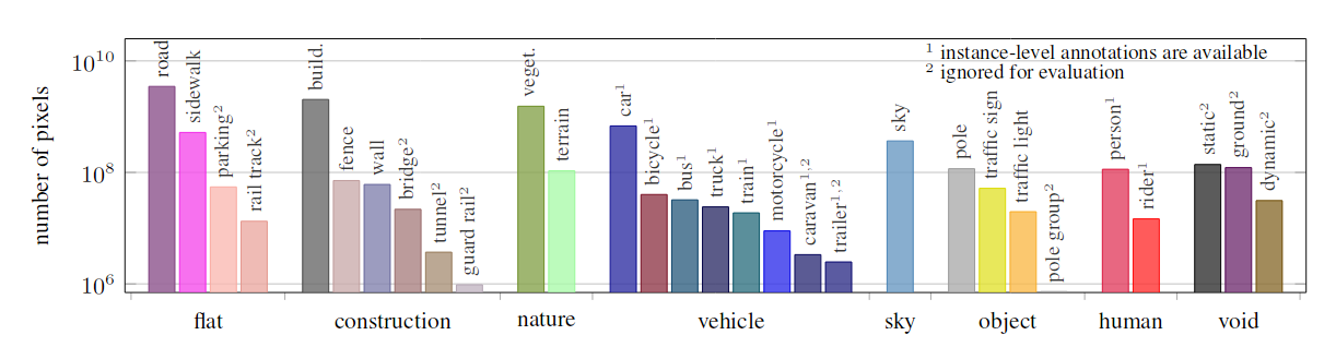
Frequency of appearance of each label in the database
Visualisation
We will represent labelled road images by attributing a color to each class. We use the following color code:
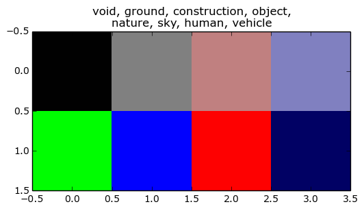
Color code for the class labels
Therefore, we can visualize a labelled image by coloring each pixel with the color corresponding to its label. Here is an example:
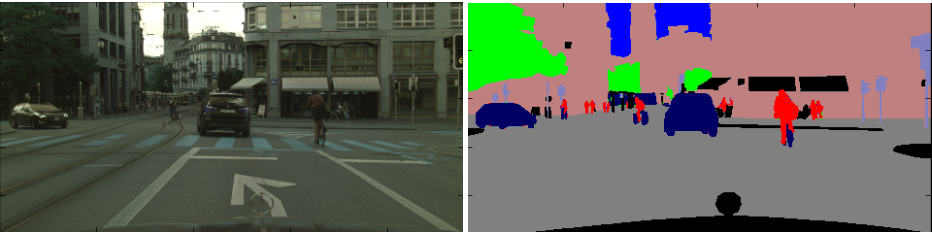
Photo (Left), Colored Labels (Right)
We will use deep neural networks to set a label to each pixel of an image. We can either work at a local scale, by looking at the close surroundings of each pixel to compute its label (Sliding window), or work at a global scale (autoencoder) to take into account the structure of the whole image.
Sliding Window
How it works
In this method, we train a classifier that takes as input small frames of size 64 x 64, and computes a label for the frame. To do so, we compute for each image in the dataset, overlapping frames of size 64 x 64, normalize them (RGB channels) and save them in a new training dataset. For instance we take, for , , the family of frames
After training, we can segment a whole image in the following manner: first, we define overlapping frames of the image.
Each frame is then labelled with the classifier, which let us assign the frame's label to every pixel in the frame. Each pixel receives many labels (because of overlapping frames), so we use a majority vote to set the pixels' labels.
For our classifier, we use the LENET architecture :
The LENET architecture. Activations are not shown.
This network is composed of convolutional layers that detect patterns in the image, of MaxPooling Layers that downsample the image to compress information, and of regular densely connected layers.
Computing the training set of 64 x 64 steps is a delicate step and conditions the efficacy of the neural network.
We choose to consider in the family of frames defined above. The goal is then to assign a unique label to each frame.
We adopted the following principle: If at the center of the frame, the proportion of pixels assigned to a specific group is higher than a threshold, then the frame is considered to be a sample of class . We chose different thresholds for different classes and consider an order in which the classes must be examined.
Say that we have a list ordered_labels of labels ordered by decreasing importance (for instance pedestrians first and void last), and a list of thresholds attribution_label_filter. We can apply the following algorithm :
- For l in ordered_labels :
- center = frame[12:-12, 12:-12]
- filter = attribution_label_filter[l]
If the percentage of pixels ofcenterthat are labelledclassis higher thanfilter, then we assign the labelclasstoframe.
If no class verifies this condition, then thisframeis not kept in the training set.
It means that for a frame to be labelled with label , the proportion of pixels in its center is lower than the thresholds associated with classes more important than .
Why don't we chose the same threshold for all labels ? The fact is, it is very easy to obtain samples of sky because images often display large regions of pixels labelled "sky". On the other hand, pedestrians are much less represented in the original images and will often occupy few pixels in an image. It is critical to set a low threshold for pedestrians in order to detect people that are quite far from the car, while it is not necessary to detect all frames containing more than 50% of sky. We can however keep those sky frames with a low probability to still allow for sky border detection.
We determine the importance order for our labels by answering the question: which labels are more important to detect ?
For the filter_attribution_label parameter, experimental tests allow us to verify if we obtain a sufficiently high number of relevant samples for each class.
We considered the following order, with filter thresholds :
| # | 1 | 2 | 3 | 4 | 5 | 6 | 7 | 8 |
|---|---|---|---|---|---|---|---|---|
| Class | human | vehicle | object | construction | nature | sky | ground | void |
| Threshold | 20% | 75% | 40% | 80% | 70% | 50% | 80% | 50% |
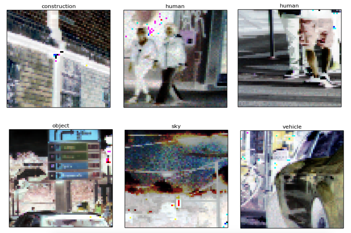
The parameters of over-represented labels (sky, ground, construction) are left to a sufficiently low value to allow for diversity. We can afterwards choose the size of the dataset for each class.
Here are a few examples of (RGB normalized) images for each class:
Accuracy
The sliding window method has been used with a LENET architecture and a dataset of 8000 samples (1000 for each class). It then has been evaluated on labelling whole images, by looking at the percentage of well labelled pixels.
| Class | Train Accuracy | Test Accuracy |
|---|---|---|
| Void | 40.3% | 14.1% |
| Ground | 63.5% | 60.0% |
| Construction | 35.7% | 29.6% |
| Object | 33.3% | 28.6% |
| Nature | 55.1% | 48.2% |
| Sky | 90.1% | 83.4% |
| Human | 48.3% | 35.3% |
| Vehicle | 54.8% | 44.7% |
| Mean | 52.6% | 43.0% |
The accuracy gap between train and test images is a measure of how complex and well defined each class is. For instance, "Void" is broad, default class, with a large train-test accuracy gap.
With a mean test accuracy of 43%, this model correctly classifies about 43% of all pixels in test images.
Visualisation
We take three images from the test set, label each pixel using the LENET network and compute a colored image from the labels. Below are the results: in each column, we show the original image, the (colored) ground truth and the colored prediction.
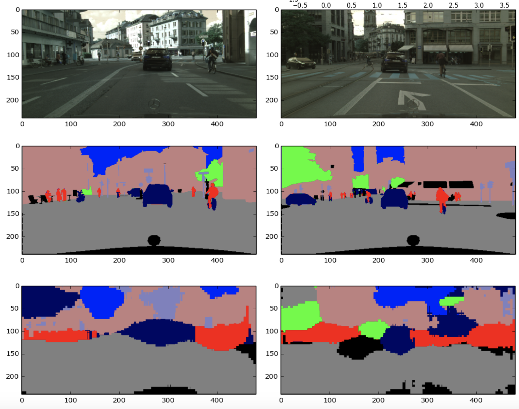
We can make many observations on these images.
First, the overall logic of road images is here: road in the bottom, mainly buildings and sky in the top.
Pedestrians are well detected, but many pixels are classified as pedestrians whereas they are just close to pedestrians, which is the reason for those large red areas around the persons. The reason for this is that we chose a threshold filter for pedestrian relatively low, yielding many frames with only a few "pedestrians pixels" being classified as pedestrians. Therefore, during the analysis of the image, the surroundings of a pedestrian will also be classified as pedestrian.
We note that many "building" pixels are classified as "car" pixels: the algorithm has trouble differencing the two classes.
A strong difficulty in the classification by sliding window is that the ground truth presented above is not analyzed as ground truth for our database creation method. To demonstrate this, we can apply a voting system to the ground truth image, for each frame of size 64*64 and then move the frames by 20 pixels each time, which gives the following result:
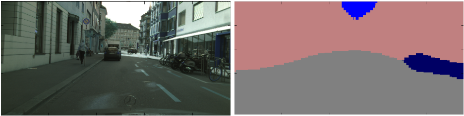
Left: Photo, Right: Voting system applied on the ground truth
The pedestrian on the left and the car are eliminated from the picture by this voting system. Hence, this method has inevitable limitations.
Direct Segmentation via AutoEncoder
Here, we will directly map an input image to its label image, through a deep Auto Encoder.
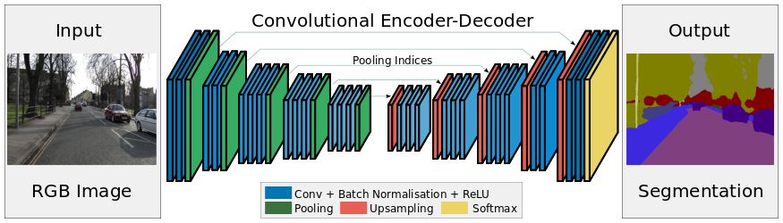
Network Architecture of an Auto Encoder
The network encodes each image into a smaller vector space (the latent space) through pooling layers and then decode it through upsampling layers.
By training the neural network, it will discard all unnecessary information about the images and only keep features that are relevant for segmenting the images into classes, because the latent space is too small too retain all the information in the images.
Here is the exact architecture we implemented, with a total number of 1,330,248 parameters.
Due to technical constraints, I was not able to use the complete CityScape dataset : The training database consists of 690 images taken in Zurich, Erfurt, Bochum, Dusseldorf and Weimar. The test database consists of 365 images taken in Strasbourg.
We trained the network with the adadelta optimizer, with early stopping to prevent overfitting. We also took into account the fact that all classes do not contain the same number of pixels : they are imbalanced. To tackle this issue, we do a reweighting in the loss function: the bigger the weight for class , the more the loss function associated to class contributes in the total loss function. The weights are computed as the inverse of the frequency of each class in the training set.
| Class | Void | Ground | Building | Object | Nature | Sky | Human | Vehicle |
|---|---|---|---|---|---|---|---|---|
| Weight | 12 | 2 | 4 | 52 | 6 | 30 | 138 | 14 |
The precision is therefore computed as a weighted mean on all classes.
Accuracy Results
The raw results is a precision of 88.5% for the training set and 84.35% for the test set.
However, we can push our analysis further with other performance indicators.
In classification, we call true positive for class () the examples correctly labelled with class . The false positive () are those incorrectly classified , and the false negatives () are the examples that should have be classified as .
- The precision index for class is computed as . It answers the question "How many examples classified as are really of class ?"
- The Recall index for class is computed as . It answers the question "Which percentage of class has been correctly classified ?"
- The Jackard index is computed as . It is the index that discriminates the best neural networks on the CityScape dataset.
The next table shows these different indicators for each class, and the obtained mean.
We can see that some classes have been learnt much better than others, despite class balancing. The 'pedestrian' class has a low recall, which mean that few pedestrian pixels are detected. On the other hand, when a pedestrian pixel is detected, it actually is a pixel of pedestrian with 62% probability.
The worse class is the class 'object', probably because it is a broad concept and there is too much diversity within the class.
| Class | Precision | Recall | Jackard Index |
|---|---|---|---|
| Void | 0.94 | 0.64 | 0.61 |
| Ground | 0.87 | 0.97 | 0.85 |
| Building | 0.78 | 0.89 | 0.71 |
| Object | 0.55 | 0.18 | 0.16 |
| Nature | 0.86 | 0.84 | 0.74 |
| Sky | 0.92 | 0.87 | 0.81 |
| Human | 0.62 | 0.27 | 0.23 |
| Vehicle | 0.74 | 0.61 | 0.50 |
| Mean | 77% | 66% | 54% |
Visualization
The autoencoder yields better visual results than the sliding window method ! Original images have been encoded in YUV format, and then normalized by setting the luminance parameter at 0.5. We can see that the overall structure is respected, and small details are much better captured.
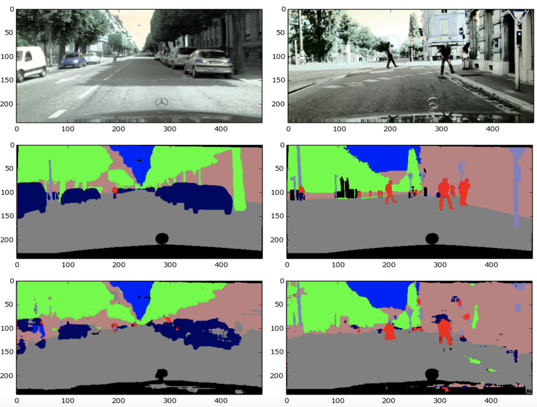
Segmentation of two images with an AutoEncoder.
State of the Art
The best network on Cityscape is ResNet-38 and obtains to this date (November 2016) a Jackard index of 91%.
Conclusion, Discussion, Further Work
That's it ! we have demonstrated how to use the sliding window method and autoencoders to perform road images segmentation. Each image takes 0.15s to process, which shows the feasibility of a real-time pedestrian detection algorithm. To build a complete tool for pedestrian detection, we could for instance scan the image with a low detection threshold. Then, we can use other algorithms to estimate their distance and their position on the road.
Our network can be improved in many ways: First, the Cityscape images are labelled with 30 classes, but we chose to group them into categories and to use only 8 classes. The reason is that extracting 64*64 frames representative of a single class gets harder when the number of classes gets bigger. Frames become less relevant and the truly interesting pixels might only cover a fraction of the frame. We used the same classes for the autoencoder, for comparison purposes; however, for this model, training on the original 30 classes will improve performance, because pixels inside each class define objects that are visually closer from one another, making segmentation easier.
Furthermore, the model has been trained on 700 images, which is relatively small given the complexity of our problem. The original training set has 4 times more images, and should be used to further improve performance. Also, due to GPU constraints, we implemented a model that is relatively small compared to modern standards.